ZTF Data Quailty Home
| Topics |
|---|
| Filterless flats. |
| Filterless LED comparison. |
| Colour response (g-band). |
| Colour response (r-band). |
| Colour response (i-band). |
| Colour response (g and r). |
| Time dependence of colour response (r-band). |
| Discussion. |
ZTF Filterless Flats
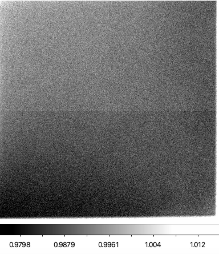
During DQ meetings there has been a suggestion that the quality of the data may be improved by performing flats without a filter. The idea being that this will remove much of the evident edge scattering as well as reflections.Below I plot the ratio of the 2020-03-09 r-band dome flat for CCD-01 to that of flat taken without a filter (pure LED).
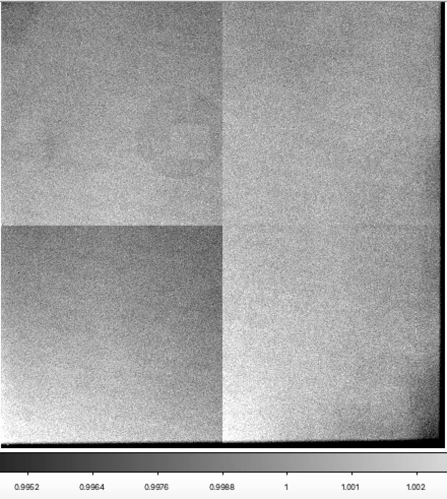
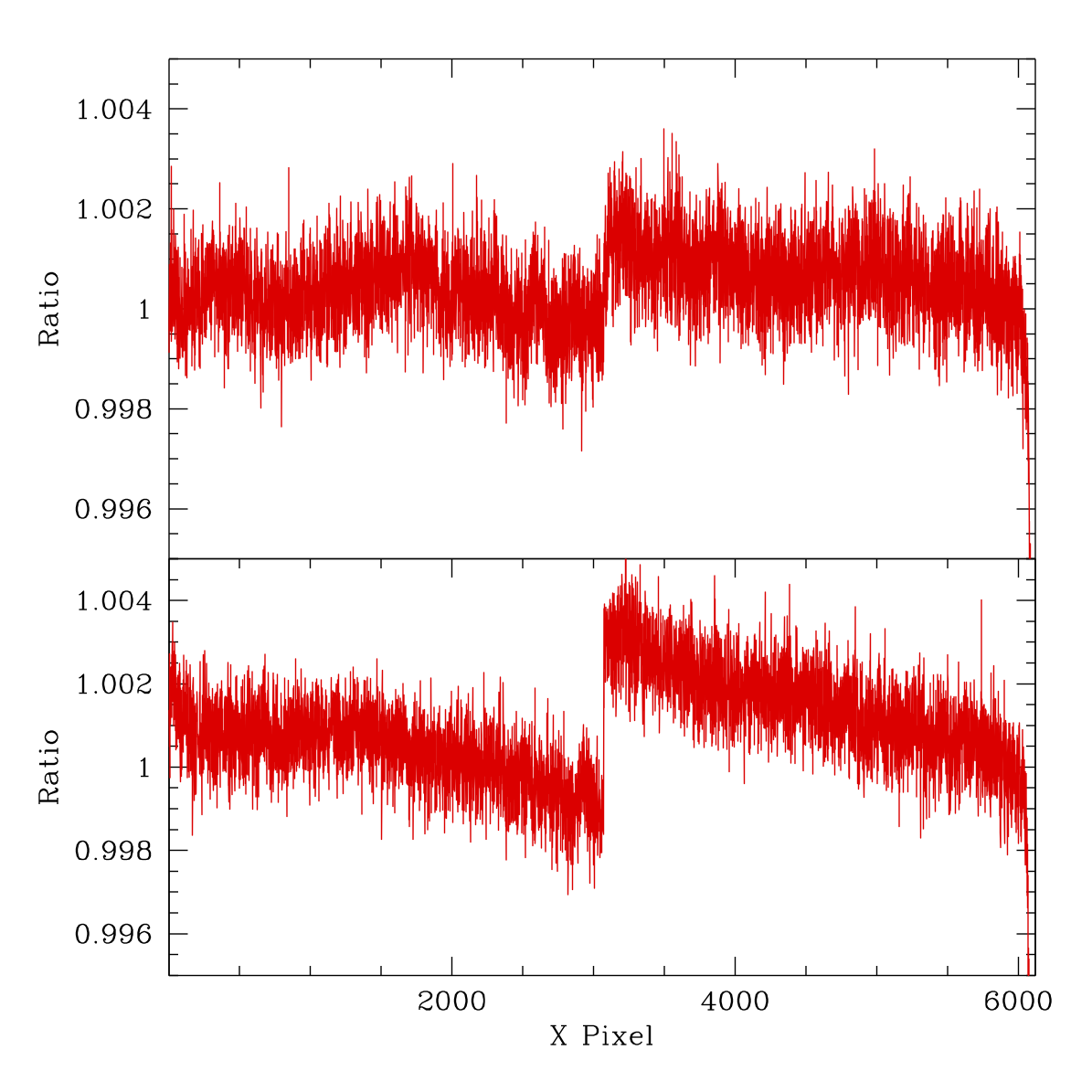
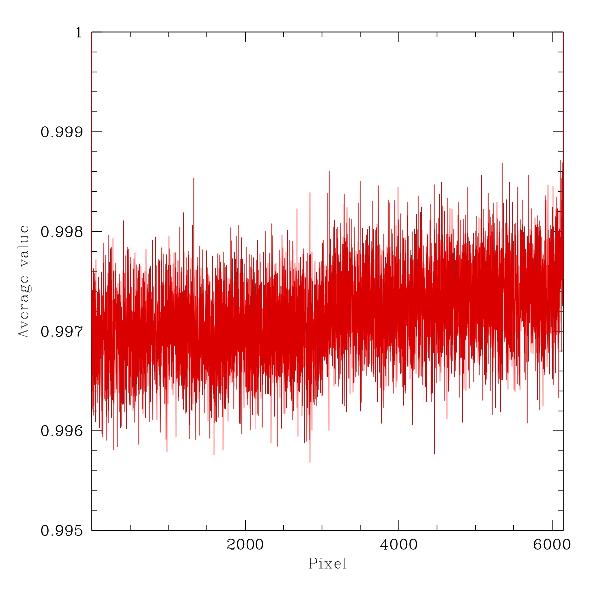
The ratio of the ZTF r-band flat from 2020-03-09 for CCD 01 to a flat without a filter taken on 2020-03-12. In the figure on the right I plot the pixel values. The top plot gives values across the middle of the top two quadrants, and the bottom the middle of the lower two quadrants.
In the case above the counts range by up to about ~0.2% across most of the image. On the edges, where scattering dominates, the values vary by up to ~2%.
In the case of g-band (below) the variations are about the same size (up to about ~0.3%). In both cases some fraction most of the non-edge differences appear to be due to the image gradients.
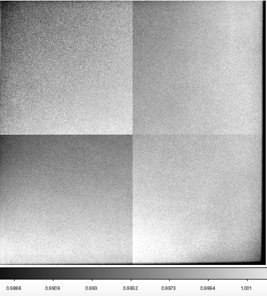
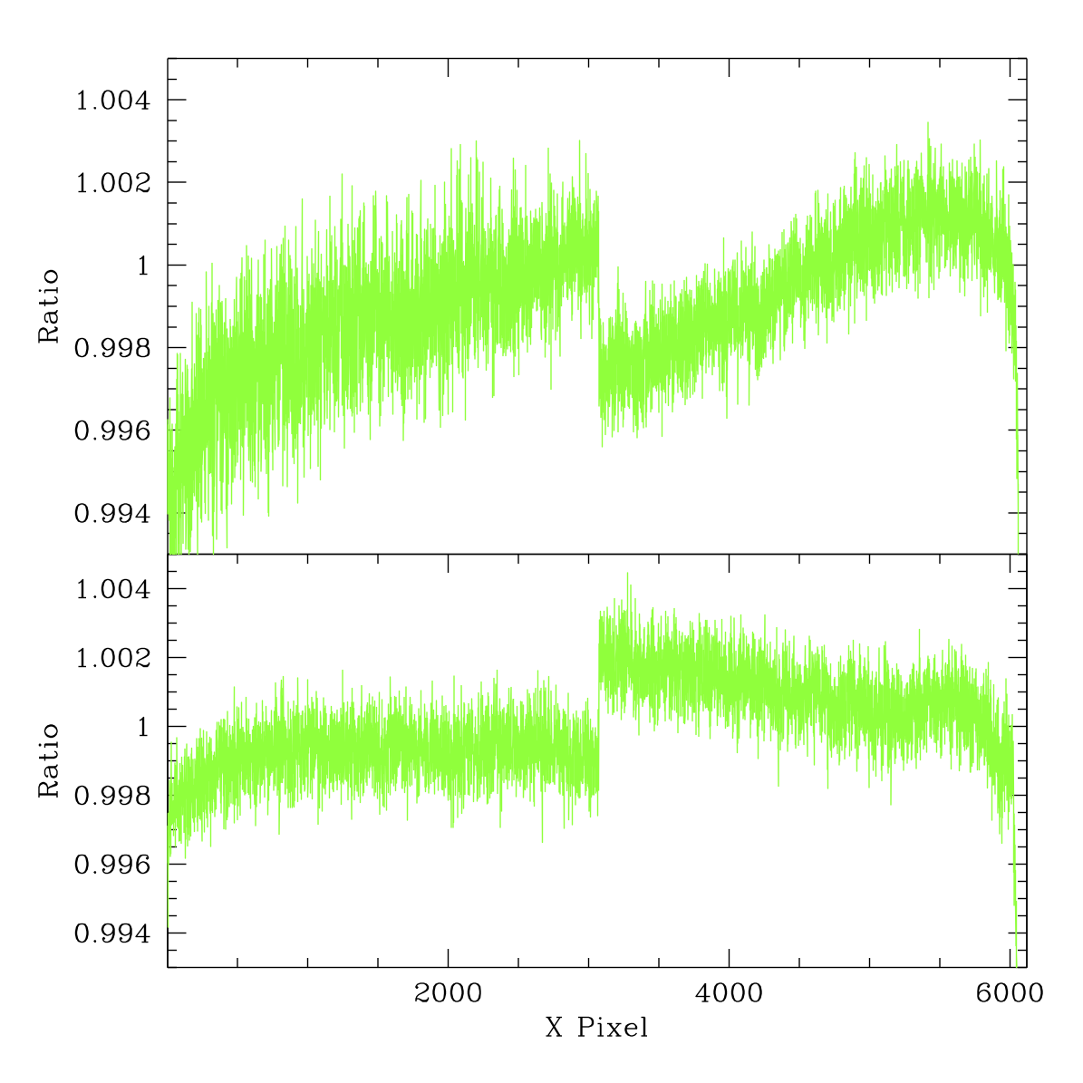
The ratio of the ZTF g-band flat from 2020-03-09 for CCD 01 to a flat without a filter taken on 2020-03-12. The top plot gives values across the middle of the top two quadrants, and the bottom the middle of the lower two quadrants.
Filterless Flats: LED comparison
Filterless flats were observed with multiple LEDs on 2020-03-12 while filtered ones in the sequence we available on 2020-03-07. We combine the unfiltered flats for each LED and then take the ratios of these to the filtered versions.
Ratio of filterless flats to g-band filtered ones for each of the four LEDs. Left top: LED #2 (450nm), Right top: LED #3 (480nm), Left Bottom: LED #4 (500nm), Right bottom: LED #5 (525nm).
Ratios through fthe our images shown above. Red line: average of lines y=4475 to 4525. Blue line: average of lines y=1475 to 1525.. Left top: LED #2 (450nm), Right top: LED #3 (480nm), Left Bottom: LED #4 (500nm), Right bottom: LED #5 (525nm).
As we can see the general structure of the images is the similar with gradients of ~1% and large edge features. The images lack any significant small scale structure. However, there are bumps with amplitudes around a ~0.1% level.
We also see that the quadrant edges in these flats are far less pronounced than in the IPAC combined flats since each is not individually normalised. The gradient in the ratio images is most extreme for LED #5. Here the flux ratio is significantly greater than the others. This suggests that the filter cuts out a significant fraction of the light from this particular LED.
Filterless Flats: colour response (g-band)
Our prior photometric analysis suggests that different ZTF CCDs require very different colour coefficients to match ZTF. This suggests that there is a varying colour response. This effect is especially evident in the case in g-band data.To consider is how the ZTF CCDs respond to light of different wavelengths (prior to planned colour calibration), we consider the spatial structure for flats taken using different LEDs. In the figures below we compare the ratios of flats taken with four LEDs within the range of the g-band filter.
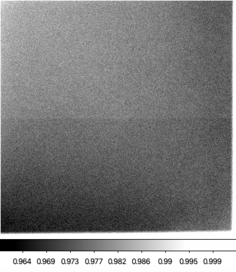
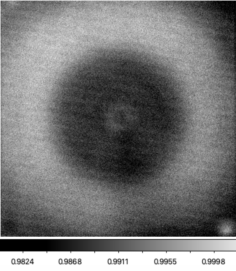
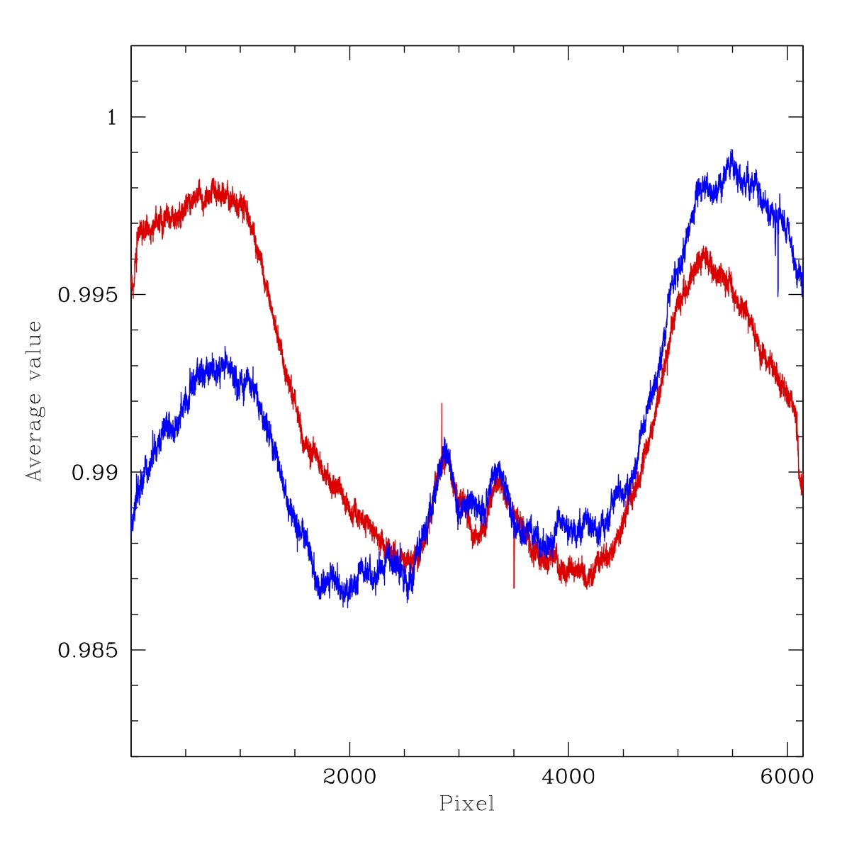
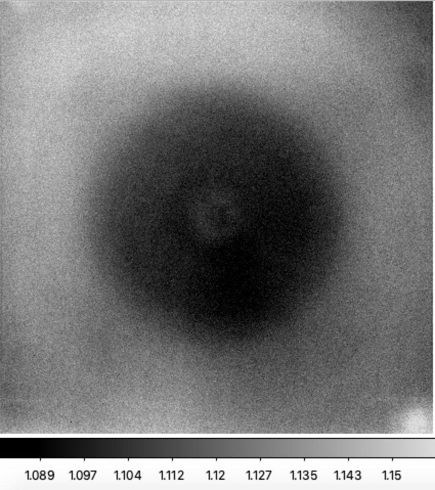
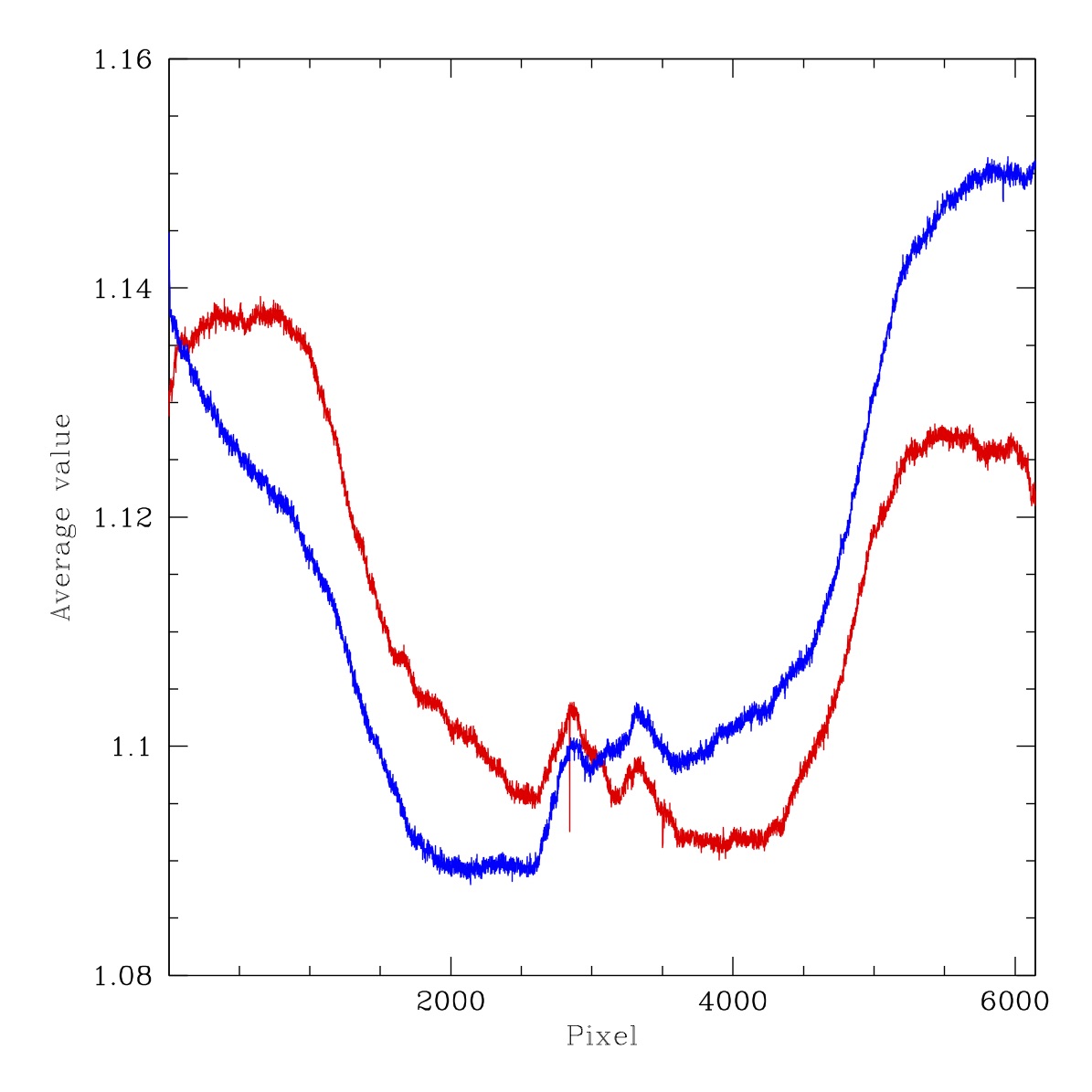
Ratio of two different LEDs for filtered and filterless flats. Left: Filtered G-band ratio LED #2 (450nm) to LED #5 (525nm), Right: Filterless ratio LED #2 (450nm) to LED #5 (525nm).
Ratios for two cuts through images shown above. Red line: average of lines y=4475 to 4525. Blue line: average of lines y=1475 to 1525. Left: Filtered G-band ratio LED #2 to LED #5, Right: Filterless ratio LED #2 to LED #5.
In the figures above we compare the ratios of flats taken with LEDs #2 and #5. These provide a moderate sepration in wavelength and thus should provide some idea of the colour dendence of spatial struture. As with many prior flats we see the diagonal lines due to the production of the CCDs. However, more interestingly we see some significant extended irregular (dark) structures that is not evident in ratio of CCDs or individual flats as well as the circular structure (due to field flatteners and CCD thickness variations?). The amplitude of the combined structure is ~1%. With an additional 1% from scattered light in the filtered images. The shape of the struture is the same in both the filtered and unfiltered cases, showing that this is not associated with the filter itself.
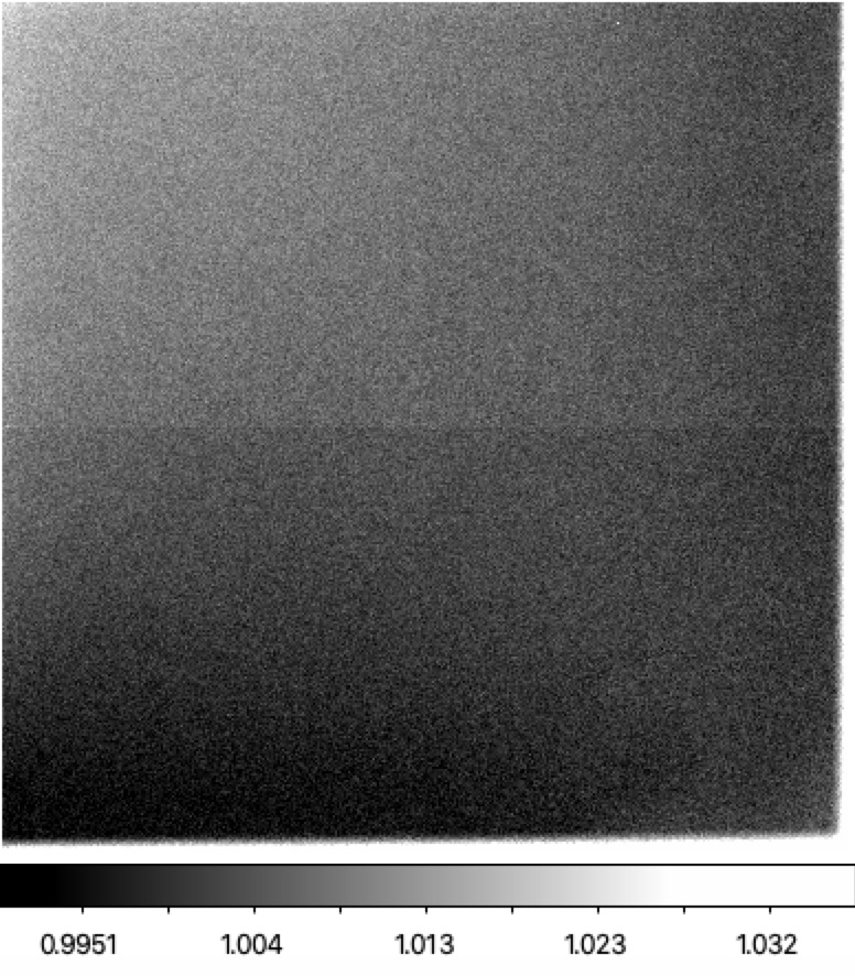
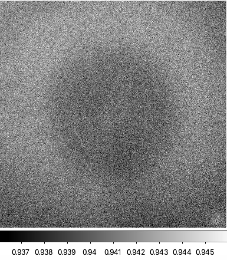
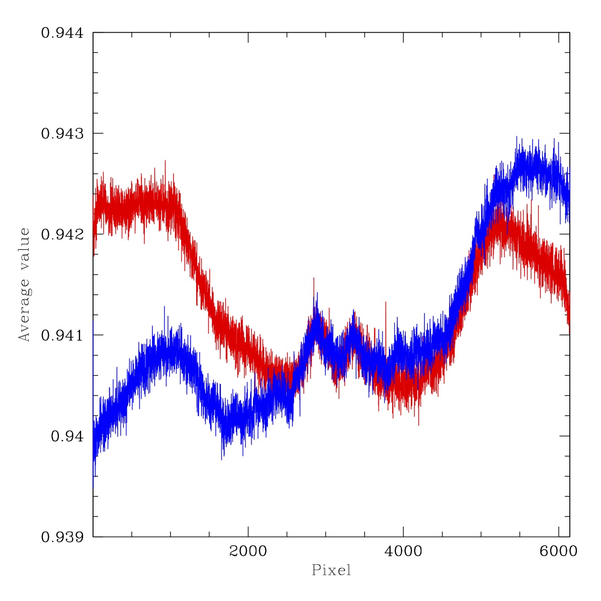
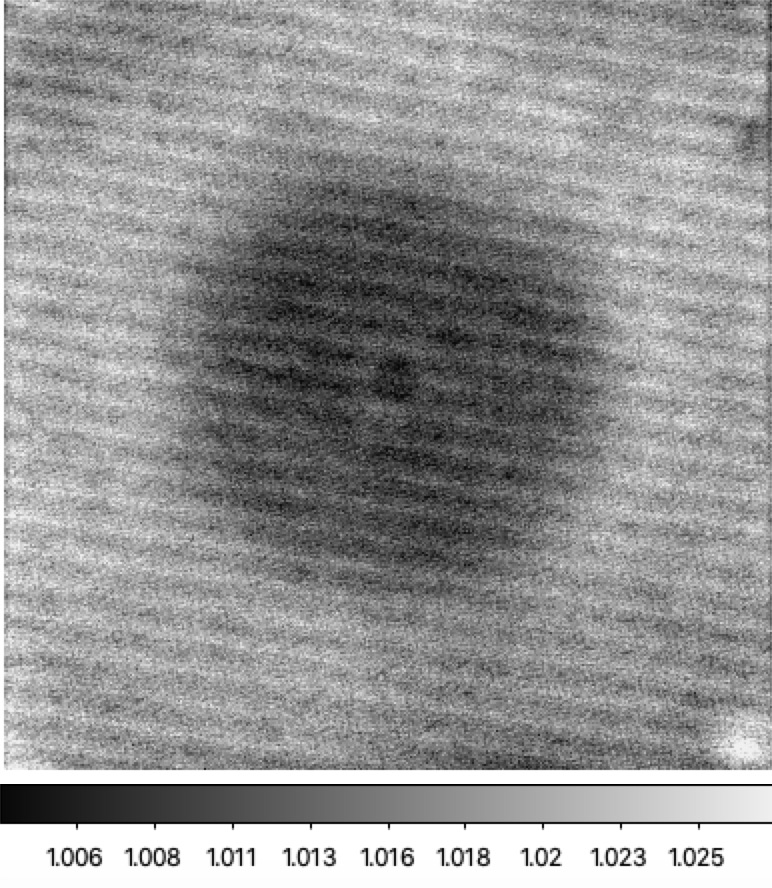
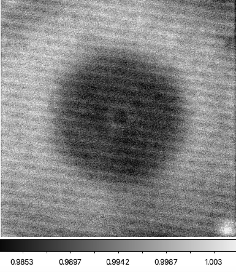
Ratio for two different LEDs for filtered and filterless flats. Left: G-band ratio LED #3 (480nm) to LED #4 (500nm, Right: Filterless ratio LED #3 (480nm) to LED #4 (500nm).
Ratios for two cuts through images shown above. Red line: average of lines y=4475 to 4525. Blue line: average of lines y=1475 to 1525. Left: G-band ratio LED #3 to LED #4, Right: Filterless ratio LED #3 to LED #4.
In the plot above we provide the ratio of LEDs #3 and #4. These two LEDs vary by only 20nm (c.f. 75nm in the other plots). Thus, they are expected to show minimal colour response variation. Here we see that the same extended structure is present, but the amplitude is significantly reduced (~0.3% c.f. 1%). This suggests that amplitude of the underlying structure is indeed wavelength dependent.
Based on the shape and distribution of the structure we suggest that this effect is due to a combination of dust (or some other residue?) with a circular colour response pattern. Similar colour dependent dust spot absorption was seen in the photometric residuals map. A ~2% effect was seen due to the accumulation of dust over time.
If the interpretation above is correct, we expect that there will be slight spatial trends in the photometry due to variations in the amount of extinction, due to dust, as well as the circular variations in response. In particular, the response to blue stars and red stars observed in the same filter will vary slightly with position. This will be add to the photometric varitions due to the colour dependence of the PSF.
It is currently unclear whether the low level spatial structure above is varying with time. However, since individual filtered LED images are available, a comparion with older images could be made.
Filterless Flats: colour response (r-band)
It is worth comparing the g-band filterless flat flux ratis above with the same effects in r-band. Here we use the four r-band LEDs 7,8,9,10 with wavelengths ranging from ~590nm to ~660nm.
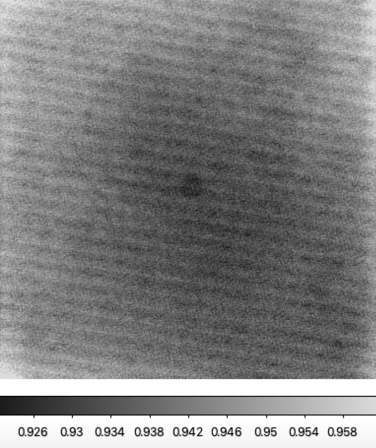
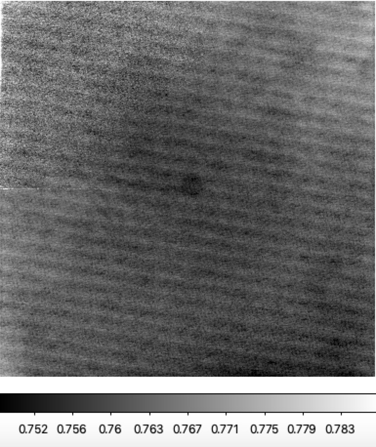
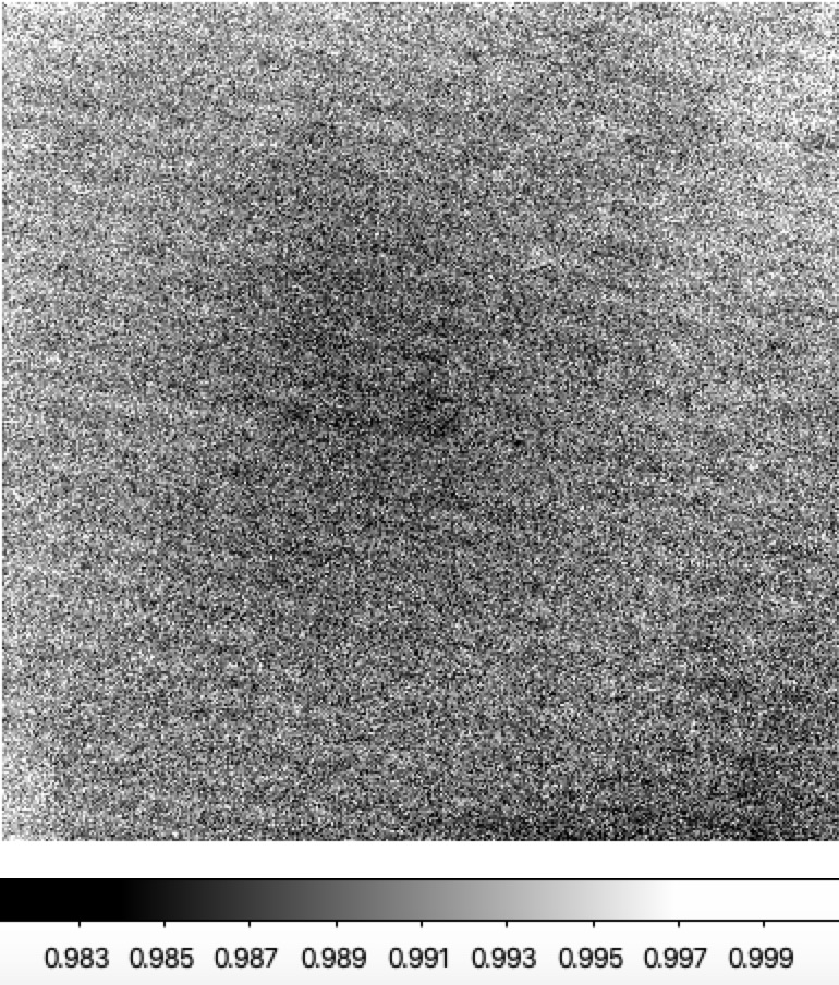
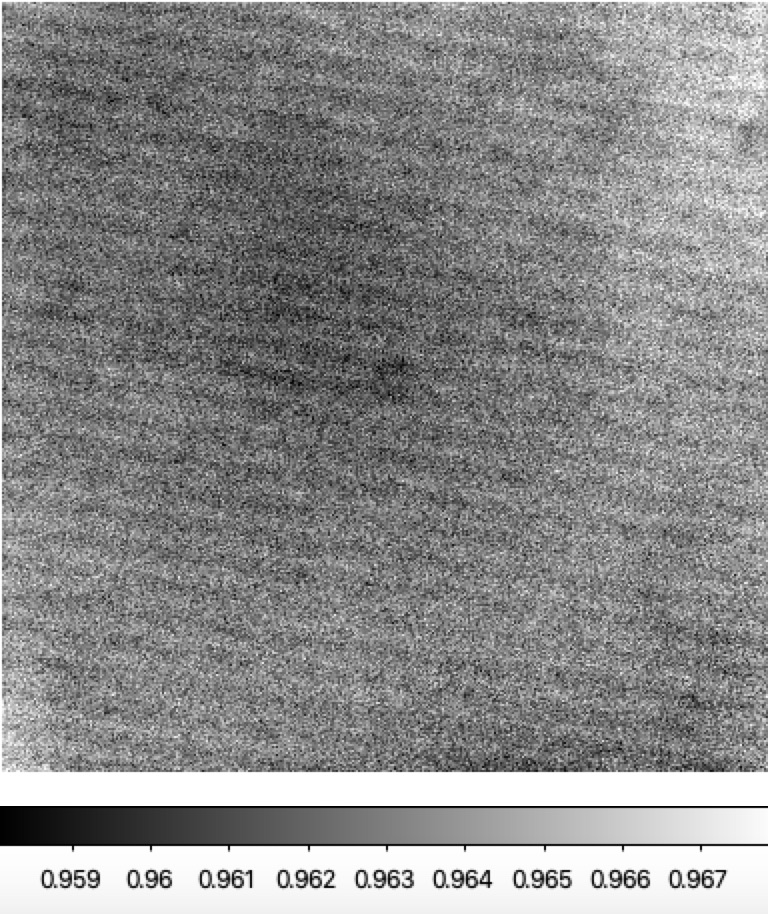
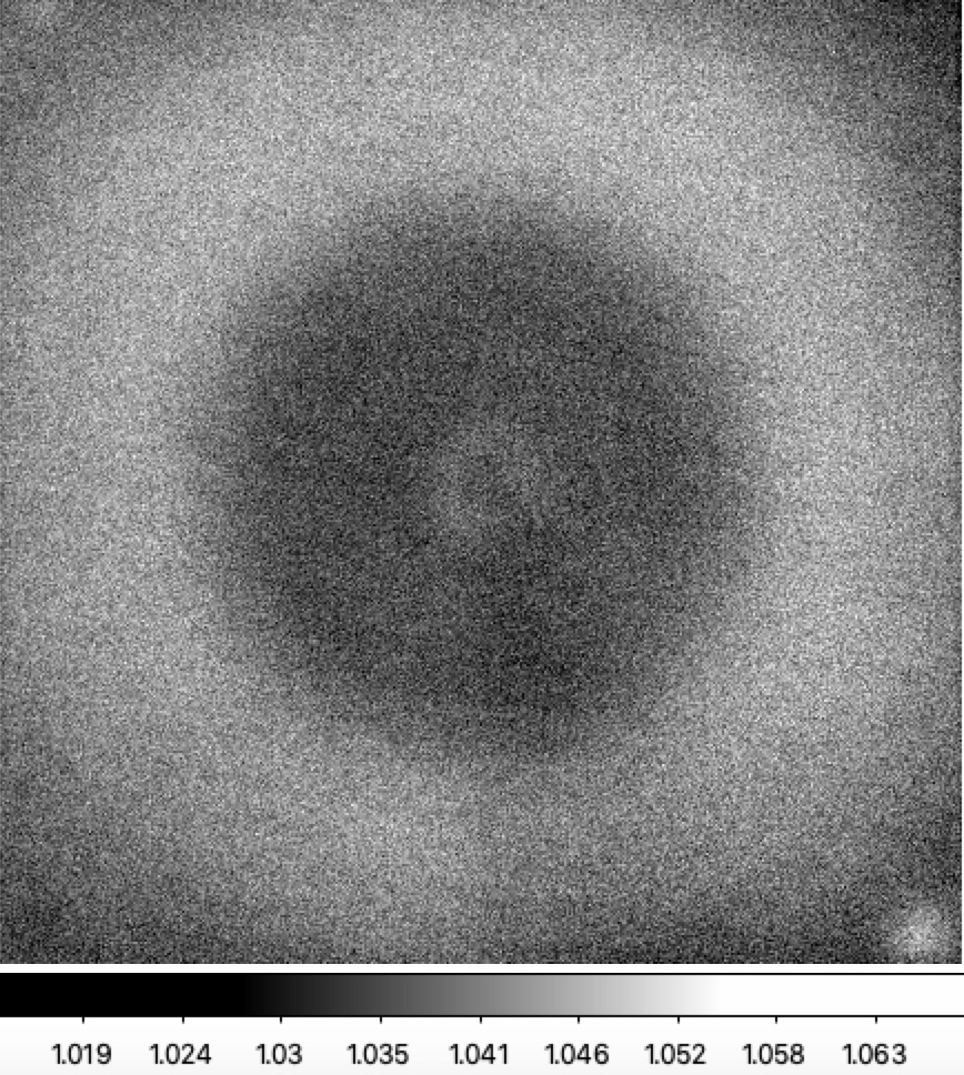
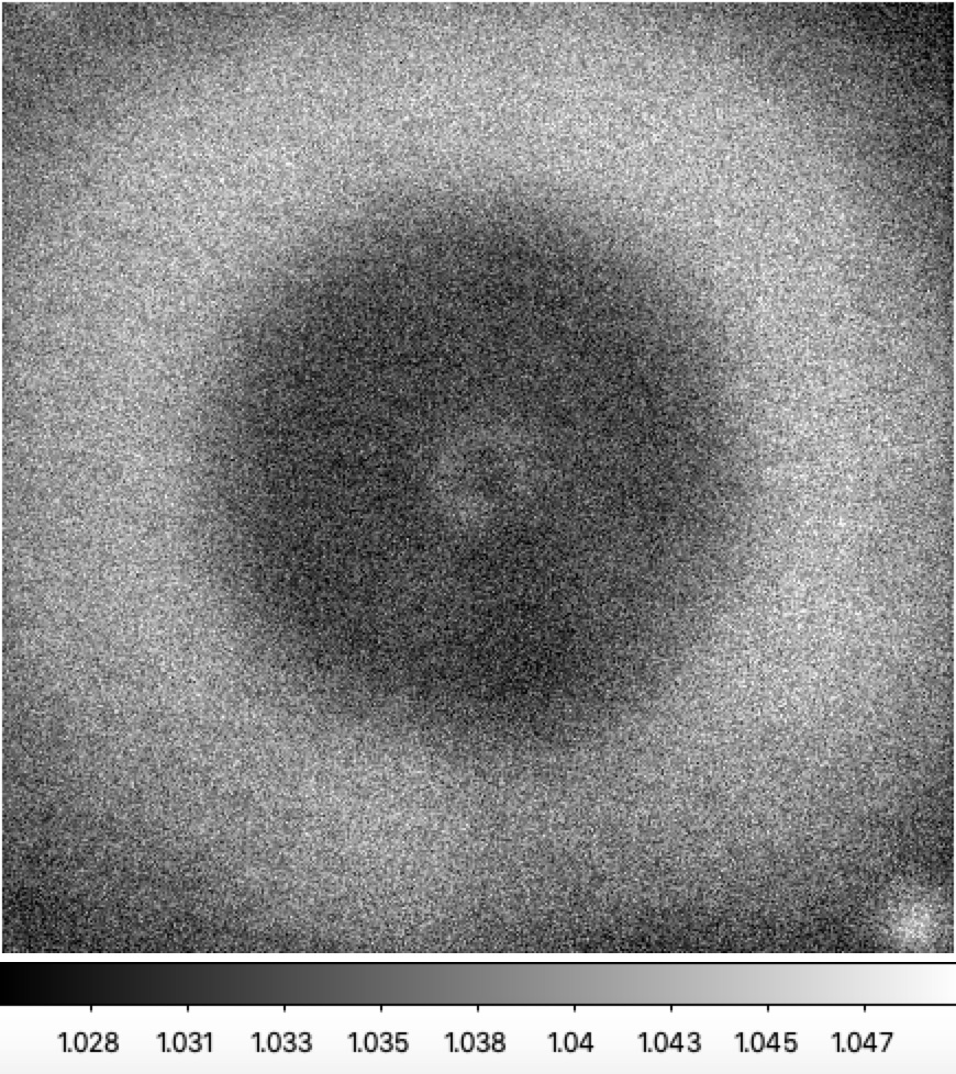
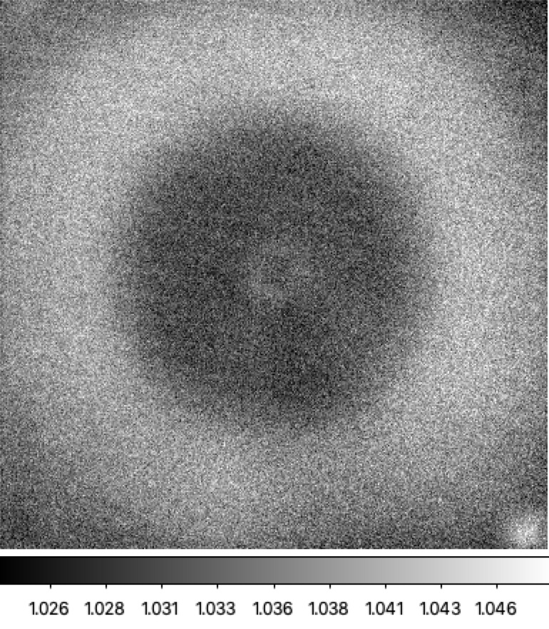
Filterless flat flux ratios for ZTF r-band LEDs. Left: ratio of LED #7 (594nm) to LED #10 (653nm), Right: ratio LED #8 (621nm) to LED #9 (633nm).
In the plot above we show the flatfield image flux ratios for r-band LEDs. As expected, the system shows a varying responses with LED wavelength. The images for LEDs in the r-band region do not show the irregular structure of the g-band image. This is consistent with the expected strong wavelength dependence of the dust induced attenuation.
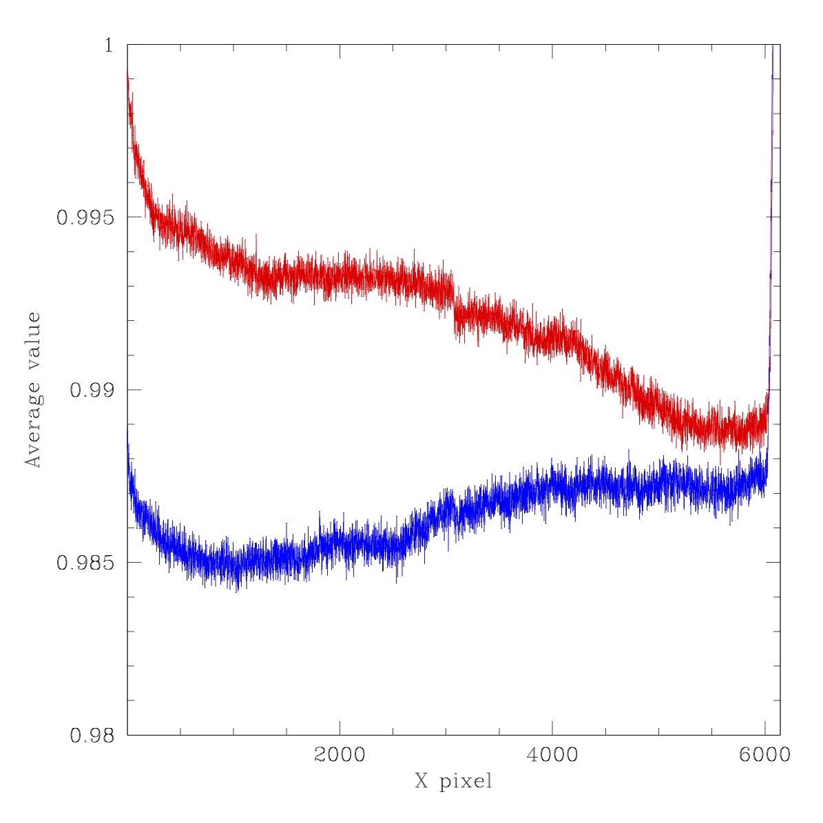
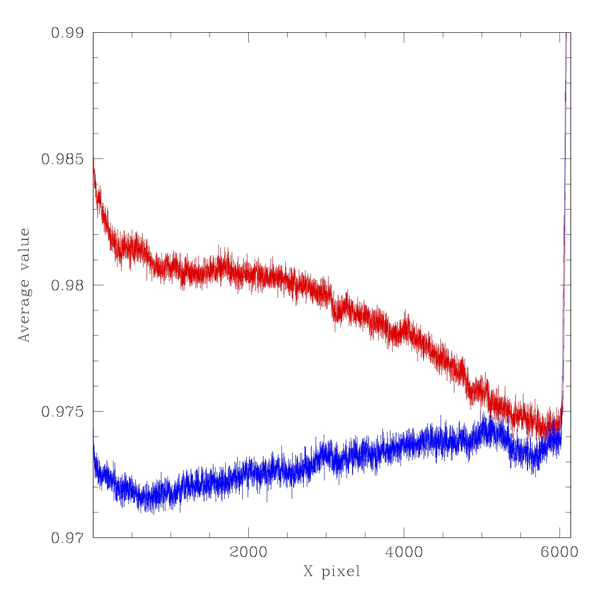
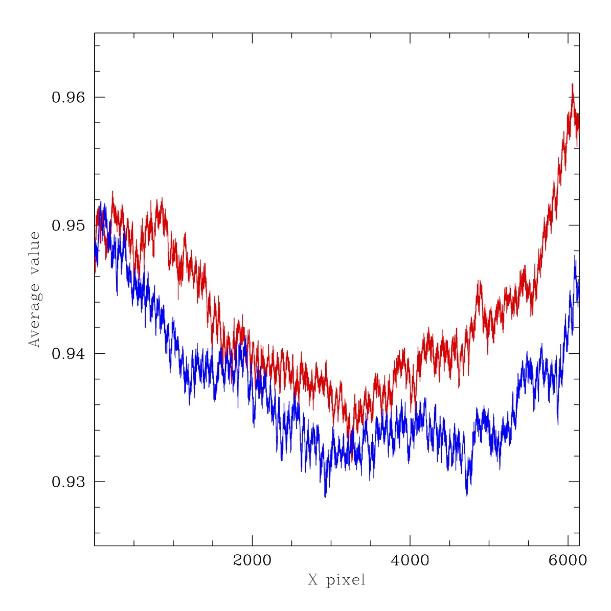
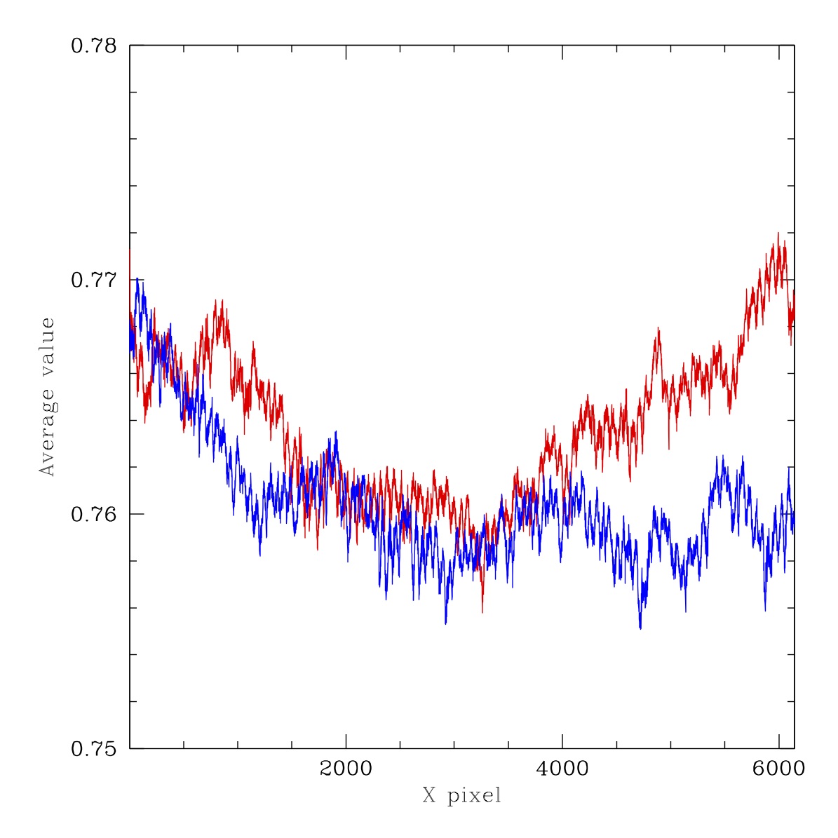
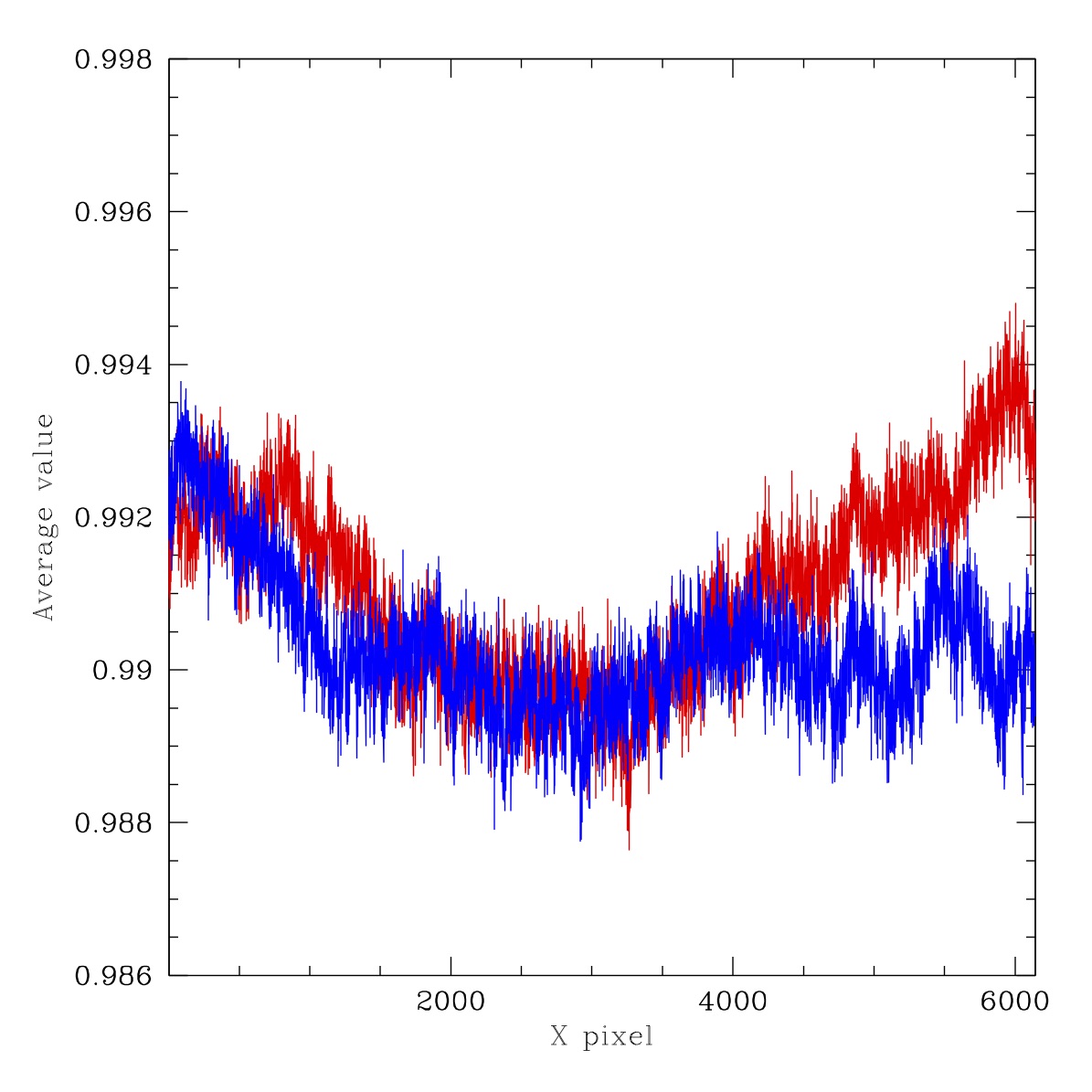
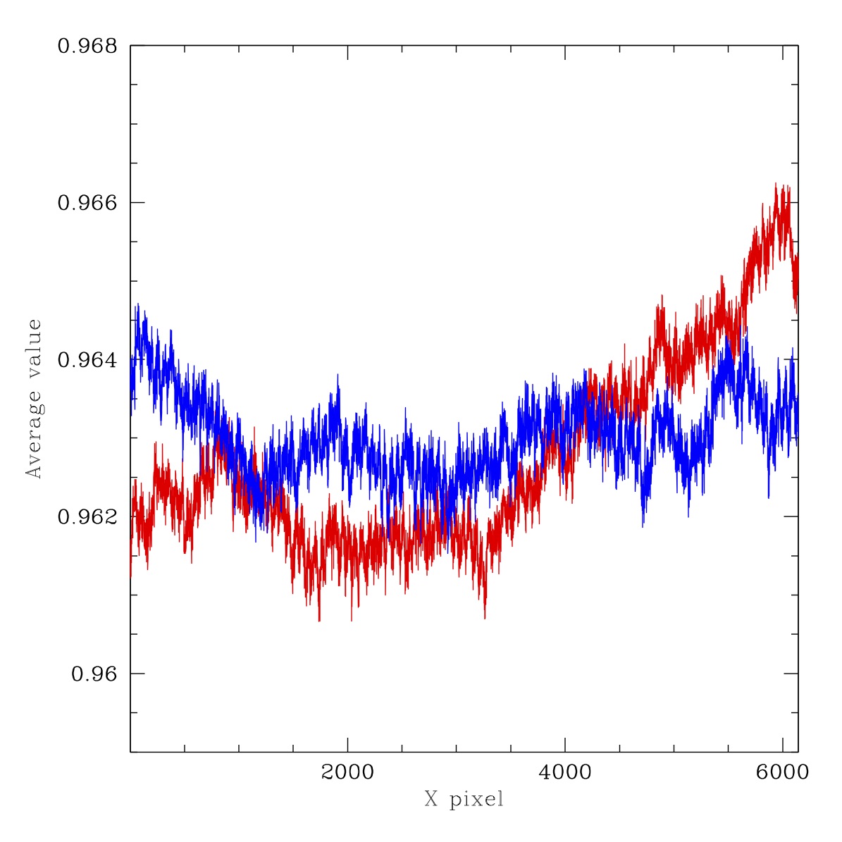
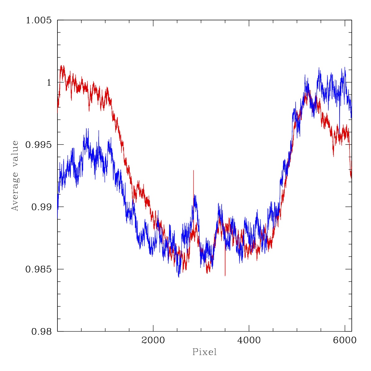
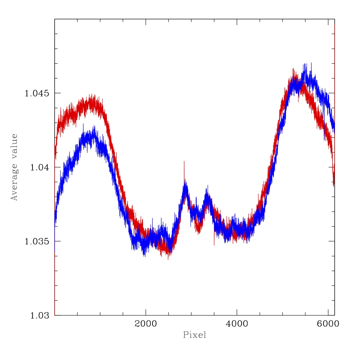
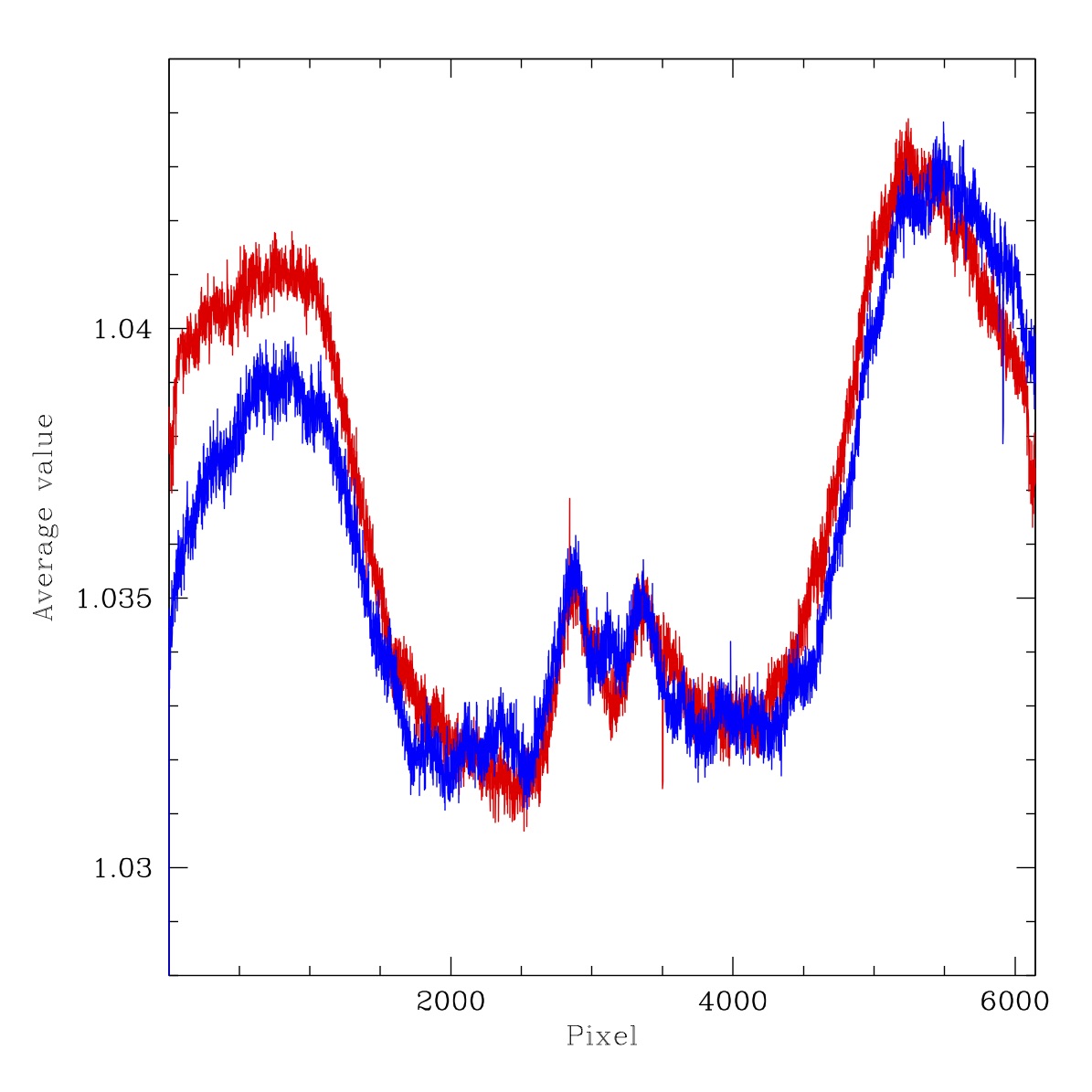
Filterless flat flux ratios for ZTF r-band LEDs. Left: ratio of LED #7 (594nm) to LED #10 (653nm). Right: ration of LED #8 (621nm) to LED #9 (633nm). Red line: Average counts in x-pixels for 3000 < y-pix < 3100. Blue line: Average counts in y-pixels for 3000 < x-pix < 3100.
The r-band LEDs #7 and #10 are separated the most (~59nm) and exhibit a 1% variation in rati as shown above. In contrast the two closest r-band LEDs (12nm separation) show a smaller (< 0.3%) variation. In the plot above we show cuts through the middle of the ratio LEDs #7 to #10 ratio image. These cuts are take both horizontally and vertically to examine the degree of symetry. Here we see that the underlying colour dependent structure is very similiar for both the closely spaced and more distant LEDs. However, the structure is not complete radially symetric.
Filterless Flats: colour response (i-band)
To compare the the i-band colour response to that of g and r-bands we have taken the single LED filtered data from 2020-04-16 for LEDs 11 and LED 13 to produce ratio images. These LEDs were at the opposite ends of the i-band filter response to determine the maximum possible effect.
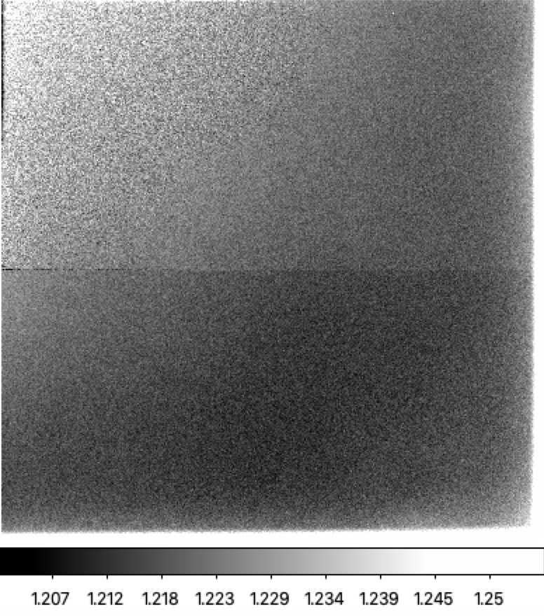
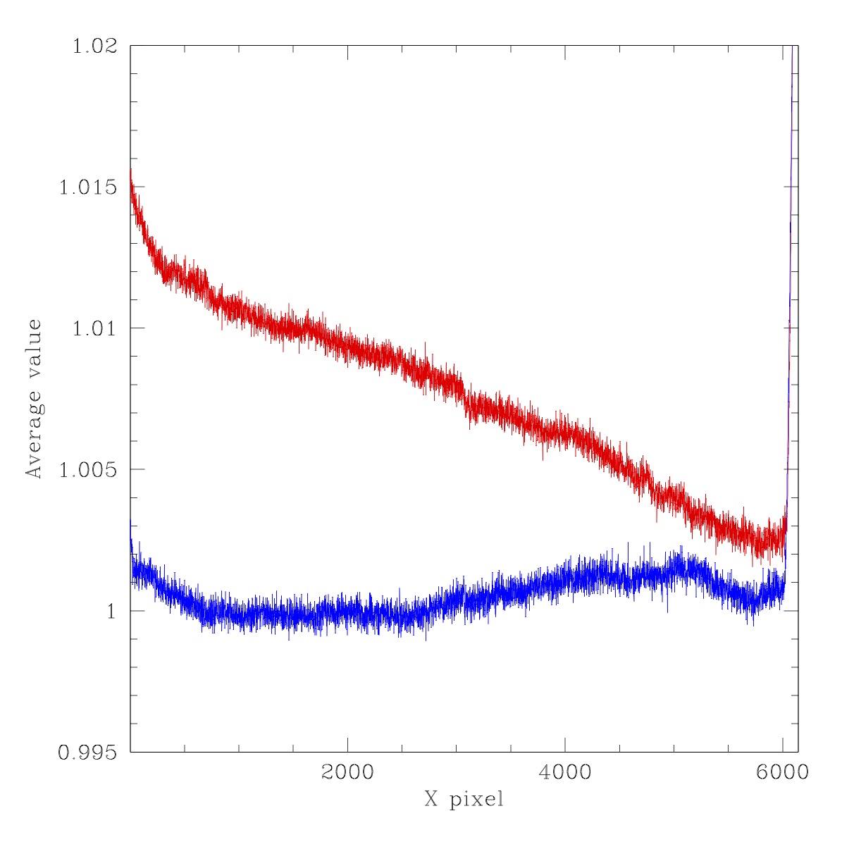
Filterless flat flux ratios for ZTF i-band LEDs. Left: ratio image for LED #11 (740nm) to LED #13 (865nm). Right: ratio counts for LED #11 (740nm) to LED #13 (865nm). Red line: Average counts in x-pixels for 3000 < y-pix < 3100. Blue line: Average counts in y-pixels for 3000 < x-pix < 3100.
Above we plot the ratio i-band LED ratio images along with vertical and horizonal slices through the center of the image. Compared to r-band the effect is much bigger (as we would expect due to increasing wavelength dependence). In fact, the effect is as large as 6% in the image. Thus this effect will be very important for i-band photometry. The wavelength difference of the LEDs used here is much larger (125nm) than the r-band and g-band ratios. So a larger effect is expected.
The shape of the colour dependency curve is similar to r-band but not exactly the same. Some of this difference is likely due to scatter light since these are filtered flats.
Filterless Flats: colour response (g and r-bands)
Filterless flat flux ratios for ZTF g-band to r-band LEDs. Left: ratio of LED #3 (480nm) to LED #6 (621nm), Right: ratio LED #4 (500nm) to LED #9 (633nm).
To see the colour dependence over a larger range we look at the variations between the g-band and r-band LEDs. For the two flux ratio images above the wavelength range is ~140nm.
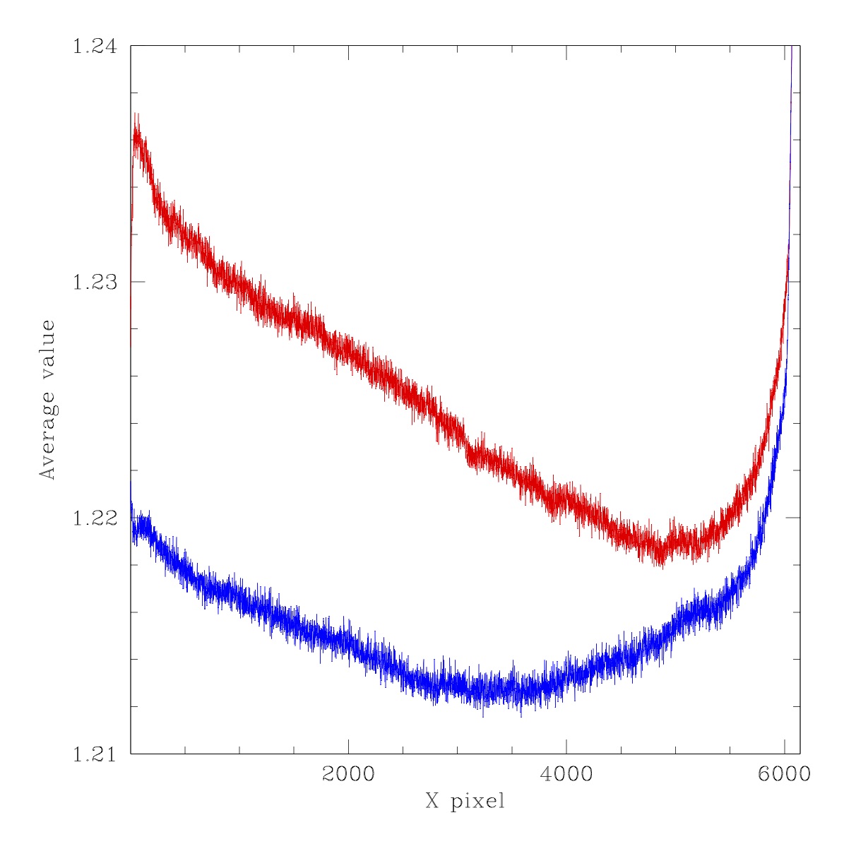
Filterless flat flux ratios for ZTF g-band to r-band LEDs. Ratio of LED #4 (500nm) to LED #9 (633nm). Right: ration of LED #8 (621nm) to LED #9 (633nm). Red line: Average counts in x-pixels for 3000 < y-pix < 3100. Blue line: Average counts in y-pixels for 3000 < x-pix < 3100.
From the plot above we see that the flux variation is around 1.4%. The shape of the response os very similar over a broad range of wavelengths. The only real difference above is from the diagonal structure. Clearly the response of the system has significant wavelength dependence that is not related to any spatial variations in the filters. However, since the amplitude of the structure only increases by 0.4% in the plot above, we see that most of the colour response variation is at red wavelengths. This is expected to be much more significant in i-band.
Time Dependence of colour response (filtered r-band only)
For the purposes of calibration it is worth considering whether the spatial dependence of the colour response has changed during the span of observations. To test this I compared ratios of single LED exposures taken on three nights (2018-08-31, 2019-09-31, 2020-04-16). These nights were chosen since the flatfield analysis suggest these nights were most likely well behaved. Only filtered flatfield images are available.Here the two LEDs chosen for the test were the r-band LED #7 (594nm) and LED #10 (653nm) since these exhibit a significant (1%) difference in response across a CCD.
Filtered flat flux ratios for ZTF r-band LED #7 to LED #10 for three nights. Left: 2018-08-31. Center: 2019-08-31. Right: 2020-04-16.
The images show the same pattern with very little to distinguish them. This suggest the spatial structure is not varying significantly with time.
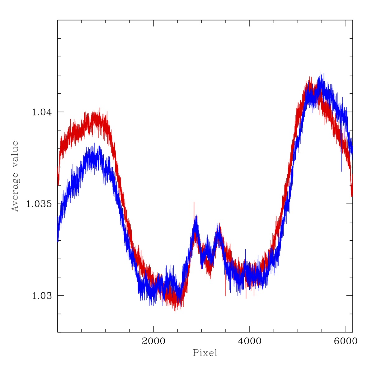
Filtered flat flux ratios for ZTF r-band LED #7 to LED #10 for the three nights above. Left to right: 2018-08-31, 2019-08-31, 2020-04-16. Red line: Average counts in x-pixels for 3000 < y-pix < 3100. Blue line: Average counts in y-pixels for 3000 < x-pix < 3100.
As a more quantitative test, above, we plot the values in the ratio images. Here we find values which are very similar appart from small (0.3%) offsets in the average LED flux ratios. The structure itself appears essentially identical. The distribution of values vary slightly (the plots are more radially symetric) from the filterless flats due to the additional scattered light.
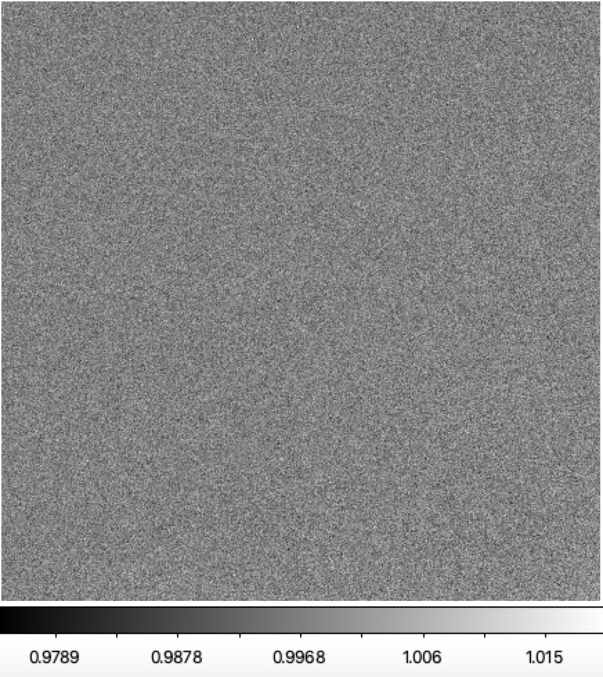
Variation of spatial colour response with time. Left: the ratio of the 2018-09-31 and 2019-08-31 LED ratio images above. Right: The average counts on the image for x-pixels and 3000 < y-pix < 3100.
To better compare the different nights, we once again take a ratio of the 2018-09-31 to 2019-08-31 LED ratio images. Since there is no structure, this shows us that there is no significant variation in underlying colour response structure on these two nights. The line plot show that there is a slight offset in the LED ratio images (~0.3%, possibly due to variation in the amount of dust extinction with wavelength) and a very slight gradient (~ 0.05%).
Overall the lack of variation in the r-band LED data suggests that the colour dependence is not changing with time. This suggest that we can accurately model the spatial colour response and correct for it.
Further work with other CCDs as well as g and i-band data is needed to confirm the current analysis.
Discussion
From the above analysis, if we consider the variations between the filtered and unfiltered flats, it is clear that there are significant differences. However, it is currently unclear how much of the gradients due to scattered light are taken out in the processing. The IPAC processed images suggest flatfield differences of order 0.5% at maximum. This effect is is much smaller than the gradient across the entire field since the flats are normalised on a quadrant level.Within the photometry, the IPAC flatfield normalization is taken out as a shift in the ZP when the data is calibrated to PS1. However, in reality the photometric zero point should vary even on scales of a quadrant. These intra-quadrant ZP differences should be taken into account by the flatfielding and are particular important on the edges of the camera where the throughput differences are significant (0.2 mags in g, 0.35 mags in r) compared to the optical center. For example, as noted elsewhere, in the most extreme cases, underlying ZP variations of up to ~0.05 mags are expected based on the variations in average quadrant ZPs between adjacent quadrants. Some residual ZP variation is expected in the photometric corrections applied to the data.
Colour Dependency
If we want to consider how much affect this colour dependency has on the photometry we should consider the difference red vs blue stars. The SEDs of these stars cause them to peak on oppostive sides of the filter bandpass. However, the emission spectra of stars do not exhibit very large differences in flux over a range of ~150nm (the ZTF g and r-band filter wavelength ranges). The largest variations in continuum are probably ~2 over this range. Thus, we expect that the effect of the colour dependence should be significantly less than 1% in the photometry of stars. In contrast, a 150nm range can be more important for supernovae and QSOs since they can exhibits strong absorption lines and broad emission lines.If we consider how this effect might manifest on the ensembles of star colours observed by ZTF, we should expect the effect to be reflected in the photometry (as per the photometric residual maps). Also, we should expect photometic residuals that shift between fields as the average star colour with the fields varies with reddening.
The colour effect is much smaller than the full amplitudes within the residual maps, since those also combined the affect of scattered light in the filtered flats, temporal trends in the flats (due to dust, etc.) and uncorrected variations in the ZPs and colour coefficients across quadrants.
Time dependency of the colour response
Our analysis above suggests that there is no significant change in the spatial colour response of the system apart from small offsets that are likely due to on-going dust accumulation.The large (2-10%) variations in the flat levels with time discovered previously are not fully understood. Some fraction is likely attributable to variations in the linearity coeffs, readout, electronics, movement of large dust spots, imperfect flatfield aligment, as well as changes in the combination of the LEDs used to produce flats.