| Topics |
|---|
| Photometric variation with Skylevel. |
| Systematic effects across the full FoV. |
| Corrections for g-band frame-level systematics. |
| Investigation of of systematics in r-band. |
The Dependence of ZTF Photometry on Skylevel.
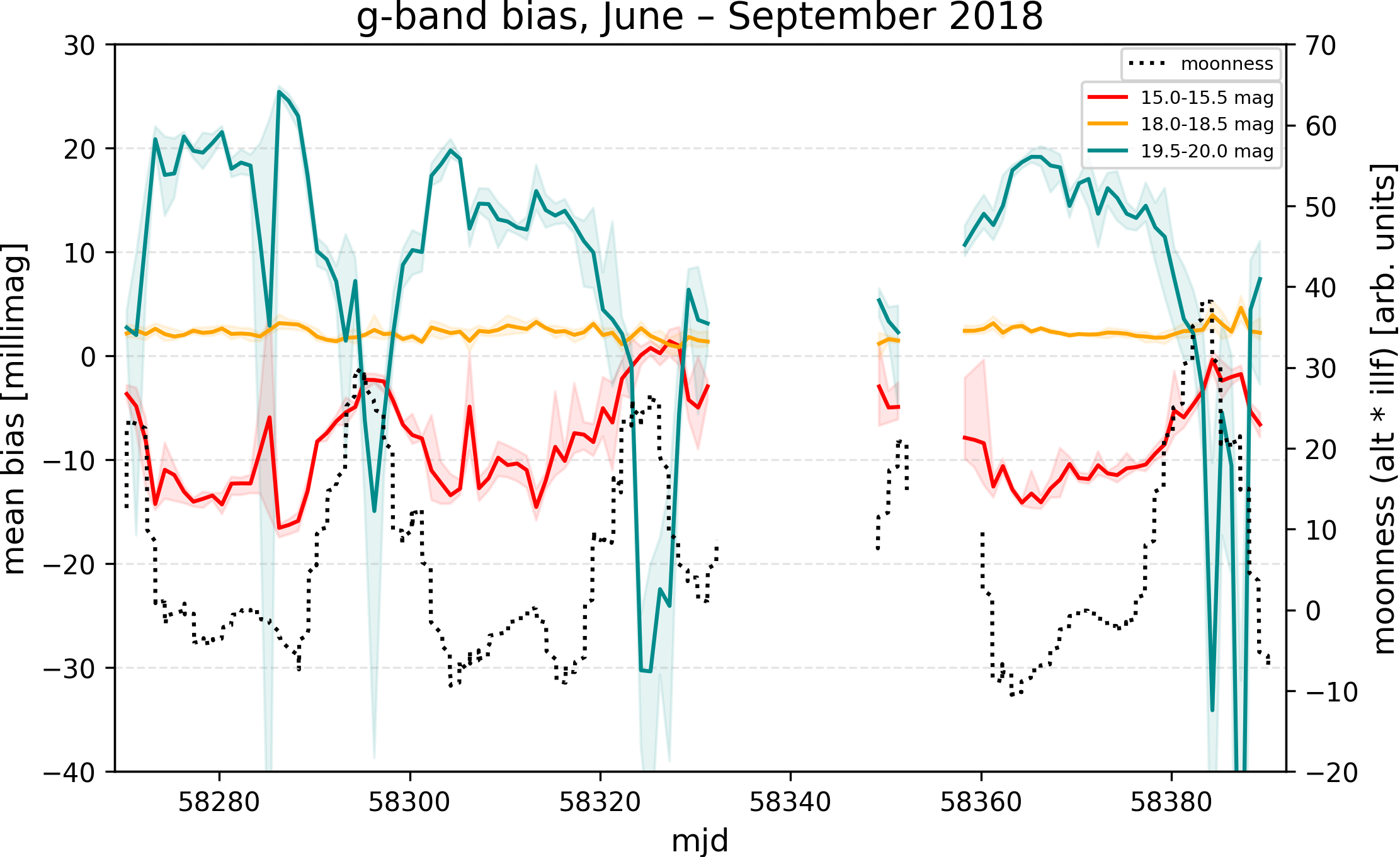
A recent plot showing problems with calibrated ZTF photometry (by Simeon Reusch).
The above plot was received from the DESY group and shows how the moon effects the ZTF calibration. This figure shows that, not only is there a variation with "moonness", but that bright and faint stars are offset to a different extent.
The most likely cause of this variation are illumination changes in the sky background level within an image (i.e. moonshine, F. Masci). To investigate how skylevel affects the photometric calibration we have calculated the average offset between ZTF magnitudes and PS1 for each individual exposures (using ZTF calibrators and ~2000 ZTF images of CCD5, quadrant 1, taken before May 2019).
This above figure shows that variations in the median sky-level do indeed produce a magnitude offset relative to PS1.
Variations in g-band magnitudes calibrated to PS1 vs sky-level after correcting for the magnitude bias.
However, after applying corrections for the magnitude bias. The magnitudes for brighter and fainter sources are in good agreement. Nevertheless, the corrected data still clearly exhibits a significant magnitude variation with skylevel.
Checking with results from multiple quadrants suggests that that the amplitude of the variation varies between quadrants. As with the magnitude corrections, this once again suggests a possible link to differences in gain response.
Skylevel effect corrected data vs the average seeing observed for a frame.
Left: Skylevel effect corrected data vs the airmass for a frame.
Right: A zoomed in version of skylevel effect corrected data vs the airmass.
Looking for effect with airmass we see that over the full range of airmass data does not show an obvious trend. However, zooming in at the low airmass region we can see some structure in the residuals.
More data is need to confirm and find the source if this airmass feature.
Variations in the skylevel dependence between fields.
From the spatial structure analysis it became clear that there we slight offsets between calibrated ZTF and PS1 magnitudes even after correcting for the magnitude and spatial structure. Thus it is natural to consider whether the skylevel dependence also varies between fields.
Average offset between ZTF mags calibrated to PS1 for individual frames based on bright stars (g < 18) in three different fields (from a single quadrant). The blue squares are from field 589. The black boxes are from field 736. The magenta cross are from field 721. The curve is the fit when all fields are combined.
The plots above show that different fields have a different response to variations in the value of skylevel. Considering these variations, I note that field 721 has 4408 stars with PS1 matches, field 736 has 12675 stars and field 589 has 48335. Thus, the scale of the skylevel dependence appears directly related to the number of stars in the field. The fields with few stars have a much strong dependence, while those with many stars have no significant dependence.
The slight systematic variations between calibrated ZTF magnitudes and PS1 for different fields noted above could be due this varying skylevel response as well as differences in the average observed skylevel.
This trend is similar to that of the ZP_rms values (above), where fields with few stars had large ZP uncertainties. Fields with more stars may have better magnitudes if there are variations in PSF, skylevel, etc., that are being better modeled due to the sampling.
The DR1 analysis suggests that ~1500 PS1 calibrators are needed per quadrant to to minimize ZP errors. Sparse fields have insufficient stars. Thus the photometry suffers and must be corrected.
Systematics seen across the full FoV
Comparison between photometric residuals and colour coefficient values for the full ZTF FoV. Left: Residuals for fields with 600 < N < 3000 stars per quadrant with g < 18.5. Right: Residuals for fields with N > 3000 stars.
Combining the full set of 64 quadrants (without correcting for internal quadrant structure or fields offsets) we see that fields with < 3000 catalog stars brighter than g=18.5 exhibit trends in residuals with both the observed skylevel and the fit colour coeff (the colour term solution used to match ztf mags to PS1). This reinforces the idea that solutions with too few stars retain biases.
Trends in photometric residuals and colour coefficient values for sparse fields (600 < N < 3000 stars) with varying skylevels. Left: Residuals for images with skylevel < 100 cts. Right: Residuals for fields with skylevel > 500 cts.
Dividing the sparse fields into high and low skylevels, we see that low skylevels give rise to low colour coeffs and negative photometric residuals and high skylevels result give in high colour coeffs and positive photometric residuals. In dense fields varying sky levels (and seeing) only cause small variations on colours coeffs and do not change the observed photometric residuals.
Overall both the sparse and dense fields are systematically slightly offset from PS1 for stars with g < 18.5 (even after correcting for the mag dependence).
Variation in colour coeff with Sky level for the full ZTF FoV. Here coeff variations are relative to a clipped average for each quadrant. Left: Residuals for fields with 600 < N < 3000 stars per quadrant with g < 18.5. Right: Residuals for fields with N > 3000 stars.
The ZTF colour coefficients show a strong depenence on sky level. Errors in the fit colour coeffs are the likely cause of the skylevel dependence of the residuals relative to PS1.
Variation in colour coefficient value with airmass.
No obvious trend in the residuals with airmass or seeing for full fields. There is a slight trend in the colour coeffs with airmass. This is expected due to the colour dependence of the second order extinction coefficient. This is about 0.015, which is about half the ususal value for (B-V).
Variation in colour coefficient value with seeing.
In addition to the other effects above, there is a bifurcated correlation between the seeing and the colour coefficient used to match ZTF magnitudes to PS1 calibrators. Unlike the skylevel, this trend is general and not dependent on the number of sources within a field. Seeing has only a small effect on ZP (0.05 mags, though field dependent).
Variation in ZP from the average in a quadrant vs skylevel. Left: The ZP and skylevel for ~120000 ZTF images. Right: Zoomed version of the figure on the left.
The figure above shows how the skylevel traces atmospheric extinction.
Interpretation:
When there is some moonlight, the presence of thin (cirus) clouds
adds extinction and decreases depth by raising the skylevel. The
ZP drops by ~1 mag as the skylevel due to the moon and thin
clouds and higher airmass (optical depth) increase 5000 counts.
When the moon isn't up, or is far from full, thicker clouds cause
high extinction without raising the observed skylevel.
In between these two extremes, moderately thick clouds and some
moonlight increase extinction and the observed skylevel.
Corrections for g-band frame offsets.
In order to correct for the offsets of g-band frame systematics seen with vary skylevel, number of calibrators (n) and colour coefficient fits, I investigated the data in a number of stages.Starting with a set of average offsets for 125,000 g-band frames, I divided the data six sets varying ranges of the number of calibration stars (n < 600, 600 < n < 1200, 1200 < n < 2500, 2500 < n < 3500, 3500 < n < 5000, n > 5000). This revealed an exponential offset with increasing skylevel. The amplitude of this effect decreases with increasing n. I fit each of the six data sets with an simple three parameter exponential.
I then investigated the how the fit coefficents for each set systematically varied with n. Then I used these priors as a starting point to fitting the average ZTF vs PS1 g-band offsets as a function of both the skylevel and the number of calibrator stars.
The residual scatter after correcting for the g-band dependency on skylevel and the number of calibrators.
After removing the trend based on this fit solution the observed offset is reduced, but is still non-zero. This is because the offset has additional systematic dependencies that affect the values of the colour coefficients for the fits. I would suggest that this means that there are systematic errors in our fitted colour coefficients. The systematic part of these errors can be at least partly corrected using the relationship between the observed skylevel and the number of calibrators we detect.
The reduction in per frame residuals with skylevel-calibrator correction.
Left: the inital distribution without any corrections.
Right: the result after correcting for the offsets using the
skylevel and number of calibrators.
We thus remove the skylevel trend and fit the variation in the corrected offsets for the trend in colour coefficents with the number calibrator stars (as observed above). Ideally a single fit that included all the parameters with systematics would be done together. However, the data is not sufficient to fully constrain such a fit (since there are observing conditions that very rarely occur), and the results below suggest this is unnecessary.
The distribution of frame averaged g_PS1 - g_ZTF values after correcting for both the observed skylevel-ncalibrator dependence and the fit colour coefficient-ncalibrator dependence. Left: The corrected sky level dependence. Right: The residual corrected for the colour coefficent dependence.
The corrected photometry does not show any significant airmass dependence as shown below.
The distribution of corrected frame averaged g_PS1 - g_ZTF values vs airmass.
To see how the corrections for the observed systematics offset are reduced I correct the data and bin the average g_PS1 - g_ZTF offsets (below).
Distributions of g-band magnitude residuals after applying corrections.
Blue line: The initial distribution of g-band frame offsets. Green line: The distribution after correcting for the magnitude bias (Gaussian fit, offset=0.002 mags, sigma=0.0028 mags). Red line: The distribution after correcting for the systematics observed with skylevel, ncalibrators, and colour coefficients (Gaussian fit, offset=0.0 mags, sigma=0.0018 mags). Note: the colours here vary from figures above.
Here we can see that, after the corrections, the 125,000 frame sample no longer has a bimodal or systematic offset, and the dispersion in offsets is signicantly reduced (i.e. sigma is only 1.8 millimags.) This result suggests that, in sparse fields, the g-band photometry for can be significantly improved by applying a correction based on the measured skylevel, the number of calibrators and the colour coefficient. However, since the correction is small, little difference is expected for faint sources. Additional work is required to see if differences between fields remain. This can be done by using sources overlapping between fields (i.e. ubercal).
Note: the variations here are calculated using all quadrants. Corrections may actually vary at the quadrant level (quite likely). Far more data (millions of frames) is required to investigate variations at the individual quadrant level.
Systematic offsets for ZTF r-band frames.
Starting with data for ~250,000 ZTF r-band frames we investigated whether the systematics trends present in g-band were also present in r-band. The first step was to see whether there was a systematic difference between ZTF and PS1 magnitudes that was skylevel dependent like in g-band.
Residuals in frame-level photometry for the observed sky level and the colour coefficients used to match PS1. Left: ZTF r-band median frame offsets from PS1 versus the observed sky-level. Right: ZTF median r-band frame offsets for PS1 compared to the colour coefficients used to match PS1 r-band.
The resulting plot shows that the data does not show any clear trend is r-band residuals with skylevel. However, compared to g-band (above) the scatter is larger. However, we must remember that there a 100,000 more frames here than g-band. Another systematic to check is whether the colour coefficient used to match ZTF photometry to PS1 shows a systematic effect. The plot above there is no obvious trend. Athlough the distribution is skewed suggesting that some effect could be present.
Colour coefficents used to match ZTF with PS1 vs the observed seeing in a given frame.
There is slight evidence for a correlation between colour coefficients and seeing. However, this is not as strong as in g-band photometry (above).
ZTF median r-band frame offsets for PS1 compared to the number of calibrator stars used in each frame. The red line shows the average value of offset for calibrators binned in groups of 200.
The next test is to see whether there is a dependence between the number of calibrator stars and residuals between ZTF and PS1 r-band. Here we see far more complex trends than in g-band. This suggests systematics in addition to effects caused by the number of photometric calibrators.
ZTF median r-band frame offsets for PS1 compared to the airmass of the observed frame.
Looking the residuals as a function of airmass we see a slight but clear trend. Dividing the data up based on the number of calibrators shows some variations. To correct the effects of airmass and number of calibators we fit a surface to the residuals vs airmass and number of calibrators.
After correcting for the systematic variations with airmass, and the number of calibrators, we found that there is also systematic dependency on the fit zeropoint (ZP) of the r-band images. The correction is only applied for ZP < 25.6 since trends at smaller values are due crowded fields (see below).
The trend in r-band residuals with ZP after correcting for airmass and number of calibrators. The red line gives the trend used to correct for the remain systematic. The dotted line gives the average per 1000 values.
Distributions of r-band magnitude residuals after applying corrections.
Blue line: The initial distribution of r-band frame offsets. (Gaussian fit, offset=0.002 mags, sigma=0.0015 mags). Green line: The distribution after correcting for the magnitude bias. Red line: The distribution after correcting for the systematics observed with skylevel, ncalibrators, and colour coefficients (Gaussian fit, offset=0.0 mags, sigma=0.0016 mags).
After correcting for systematics effects with the airmass, number of calibrator stars, and ZP, we are able to remove the slight systematic offset of the r-band frames from PS1. However, unlike in g-band, our corrections do not reduce the overall observed scatter. The core of the distribution appears Gaussian with scatter slightly less than g-band (1.6 vs 1.8 mmag).
Additionally, in comparison to the corrected residuals in g-band (section above), there is a more significant broad component with an RMS of around 5 millimags. This is not correlated with the usual observables (skylevel, ZP, number of calibrators, airmass). Instead this was found to be due to the fields being at low Galactic latitudes (or in proximity to the Galactic bulge).
Distributions of colour coefficients and Zero points for frames colour coded by their r-band residuals. Blue squares give frames with average residuals < -0.01 mags, and red squares those > 0.01 mags.
For the fields with large residuals, a clear trend between the residual and a frame's colour coefficient is observered. As shown above, on average, frames with residuals < -0.01 mags have larger colour coefficients than those with average residuals > 0.01 mags. However, most of the colour coefficients and ZP values are within the range of the much larger set of "good" values found in less crowded fields. This suggests crowding criteria may be required to correct remaining biases.