| Topics |
|---|
| An Overscan Issue. |
| Overscan Analysis. |
| Finding Bad data. |
| Overscan Variability. |
| Initial Conclusions. |
| Bad overscan fractions in All Fields. |
| The affect of bad overscans on photometry. |
| Selecting good photometry. |
An Issue with Overscans
In mid-Dec. 2019 K. Burdge noted that there was poor photometry for an object in ZTF field 848 that was inconsistent with that from overlapping field. The cause was subsequently traced to a problem where many of the science frames had negative backgrounds even though the values on the raw data appeared normal. This was subsequently traced back to problems with the overscan subtraction in the images by F. Masci. An example of a science frame and the overscan are shown below.
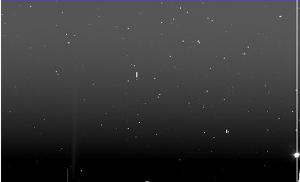
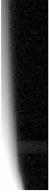
Example of an image with an unusual background along with its associated overscan region.
Overscan Analysis
To analyze this F. Masci provided overscan metrics (max,min,RMS,median,fit_rms) for all frames in the affected field (848). This consisted of 89100 sets of frame values (from ~1400 exposures).Investigation of these overscan numbers revealed very high maxima (at saturation) and high residual overscan RMS in the images with bad data. However, there were also cases of high overscan maxima when the fits residuals were small (as shown below).
Overscan region maxima vs the RMS of the overscan fit residuals. Left: full range. Right: zoomed version showing range of expected good overscan fits to the left of the red line.
There fact that there are evidently a large number of cases where overscan maxima are high, yet residuals are small, shows that the high maxima do not necessarily affect the overscan fits. Thus a high overscan maxima by themselves cannot be used to discriminate cases of bad overscan subtraction.
The occurrences of large maxima may be cases where high count values are limited to the first two columns (that are not combined in the overscan fit). Another possibility is that the high values are limited in extent within the overscan.
The overscan regions are cut from the archived raw ZTF data. It is thus not possible to tell the cause for sure without access to the images. However, I find that there are 2646 examples where the overscan maximum is > 30,000 and the fit RMS residual is < 0.7 (a good value based on the plot). Of these 2625 are from 2018 and only 21 are from 2019. This strongly suggests that the cause of the high values is not some randomly occurring event. Furthermore, it suggests the cause is not charge spillage, since that problem was not fixed until October(?) 2019.
Investigating this matter further I find that there are 29221 cases (64% of all the 2018 frames) where the overscan maximum was > 1000 cts in 2018 (with the fit residual RMS was < 0.7), while there are only 1325 frame from 2019. This strongly suggests some of the exposed pixels were in the overscan region in 2018. The 1325 frames from 2019 are most likely due to charge spillage artifacts near the edges of the overscan after the overscan trimming was corrected.
Overall, the most likely reason for the large numbers of high maxima in 2018 is that the overscan was trimmed incorrectly such that some of the exposed area was designated as overscan.
Finding the bad overscan data
Inspection of the images associated with bad photometry suggested that overscan fit RMS > 500 were generally bad. However, the plot of maxima show a large range of fit values and it is likely smaller values can also produce bad photometry to some extent. For example, another feature of the plot above is an group of values with maxima from ~100 to ~300 that have overscan fit RMS values > 0.7. This leads to a number of questions:
1, Are the smaller (0.7 < RMS < 500) values also associated with bad photometry?
2, If so, how bad is it?
3, Is there a threshold we should apply to flag data?
4, Should we correct the science images with bad overscans?
5, If so, how?
In order to find frames where bad overscan determination might affect the photometry I decided to look at the distributions of additional overscan statistics.
The left plot above shows that data with clearly bad photometry (fit rms > 500) is characterised by a large overscan RMS (>1000). However, we also see values from the second lower threshold group above. Here the initial overscan RMS and the fit RMS are very similar. This suggests that these are examples where the fits failed to reduce the scatter.
When we compare the RMS to the median frame value (right plot) we see numerous examples where the ratio is much larger than expected (< ~1). As noted above, many of these cases may be where the observational pixels are within the overscan region. Thus, we cannot select bad data based on pure high overscan RMS or an overscan RMS to median ratio.

The failure of a small fraction of fits to reduced the observed scatter in the data is even more evident in the above plot. I expect frames with even a moderate fit RMS to lead to poor photometry to some extent (i.e. particularly when an accurate background level is important).
When we look at the distribution of overscan median values we see that the are strongly grouped even when the fits themselves are very bad. This suggests that the medians are robust enough to replace the fit values in cases where the fits are bad, i.e. the overscan regions are never completely dominated by backstreaming. Since the overscan columns are fitted with quadratics simple use of medians will not be ideal. Nevertheless, they should be far superior to bad fits.
Overscan Variability
To see how stable the overscan medians are; how well they might substitute for fits, and what replacement threshold might be used, I look at the scatter in overscan median values over time.
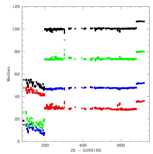
In the left plot above we see that the early data exhibited large variation on median overscan values suggesting poor data. Recent modifications to the gains shifted all of the overscan median values in the plots. In the right panel, we see that variations in the overscans during the entire stable period were generally less 2 counts. Within any given night the scatter is generally < 1 count.
Initial Conclusions
The large fraction of frames with very high overscan maxima is likely due to poor trimming of images in 2018.
Considering the above results, I suggest that RMS values for the fit residuals should generally be less than 0.7 counts. Frames in this range account for 93.5% of the data for this field (848). Significant variations are expected between fields since the worst cases are caused by highly saturated stars that happen to produce charge spillage ghosts within the overscan region.
In cases where the RMS values > 0.7 we should consider replacing the fits with the median values. However, if there are significant variations in the fits along a column, a more ideal solution would be to replace the overscan fit with a "median fit" solution offset to the current observed median value.
Since the process of replacing the overscan could take considerable time an effort, it may be a good idea to set a flag for frames with RMS residuals > 0.7.
Further analysis is required for a number (>10) other fields to determine whether the 0.7 threshold is generally reasonable and the extent of this effect on photometry. The exact level at which we flag/replace bad overscan fits should probably be decided on by the amplitude of quadratic fits and the degree of variation. I currently do not have any of the fit values.
Photometric results twenty one fields.
To verify the initial results, overscan metadata for twenty additional fields (those selected for variable star analysis) was extracted. Based on field 848 and these twenty additional fields I found that overall ~6% of this data was affect by bad overscan fits. based on a residual fit RMS > 1.The overscan data was combined with the photometry for those fields. I then selected the quadrants in those fields which had many high values of overscan fits RMS (since bad overscan fits are limited to a small set of quadrants with very bright stars). I then separated the exposures with bad overscan fits (fit rms > 100) from good overscan fits (fit rms < 1). We match the source to PS1 and compare the measured calibrated magntiudes.
The plot above shows that the scatter in photometry is not strongly affected by the presence of bad overscan data (which suggest bad fits and overscan subtractions). In fact, the exposures with poor overscan fits (high RMS) actually have fewer outliers. This result was found in multiple quadrants and suggests that poor overscan fits contribute little bad photometry. That is to say, only small numbers of sources are effected.
Fraction of Bad Overscans among all ZTF Fields
Expanding the selection of overscans to all fields I find that 4.9% of observations have overscan residual RMS > 1 (or 1164209 of the 23779536 ZTF frames). The distribution of values over all fields shows significantly higher fractions of bad overscans in fields toward the Galactic plane. This was expected due to the concentration of bright foreground stars in those fields.
The spatial density distribution of frames with bad overscans values.
The colour scale here ranges from 1% (dark blue) to 15% (dark red).
The worst fields are 333, 803, which have 22%, 17% bad overscan values, respectively.
Selecting Good Photometry
The original data that lead to the discovery of bad overscan data was a lightcurve that showed significant negative dips (suggesting an eclipsing binary) that were clearly not real. Here we present the photometry vs the overscan fit rms values for two of these objects in field 848 (CCD 13, quadrant 1, r-band) that were affected in this way.
As we can see the presence of poor overscan fits (large RMS) does not necessarily lead to bad photometry. The reason for this is likely that, as long as the backgound of a source is relatively smooth across the apperture, the flux measurement is OK even if the background is over subtracted. However, if the background changes rapidly the fit and resulting photometry will be inaccurate.
Earlier work had suggested the the reduced chi square fit of the PSF was a strong disciminator of bad photometry. Hence we look at this values for the two lightcurves above.
In the above figure we see that the poor fits values strongly correlate with deviation from the expected values. At chi < 3, the photometry is generally consistent.
To further investigate how bad data may be found we look at all the photometry for sources with r < 18 in the quadrant affected bad overscan data (Field 848, CCD 13, quadrant 1, r-band). We match each source with PS1 photometry and look at the scatter.
In the plot above we see that only a small fraction of sources exhibit the trend in magnitudes with very large chi values (> 10). The right figure shows that there is significant agreement between PS1 and ZTF photometry for chi < 3. However, there is significant tail of data that shows a fainter PS1 magnitude. This is probably due to PS1 data being less blended than ZTF.
Investigating the spatial distribution of the sources with (r_ztf - r_ps1) < 0.1 suggests that the are more commonly on the edges of fields. Looking the spatial chi distribution it was found that the edge sources had higher average values. This is consistent with the edge sources having greater scatter as found earlier.
To investigate whether the distribution of magnitude variations vs chi from the single filter and quadrant for fields 848 was similar for other filters and quadrants, I extracted the same data for all quadrants of Field 296 (in both g and r).
The field 296 photometry and chi is similar to the field 848 photometry but does not exhibit the tail of positive values related to the bad overscan fits. The g-band and r-band distributions are similar. In both cases there is the suggestion of good photometry (|mag_ztf-mag_ps1| < 0.1) for chi values up to 3 or more. However, a large number of bad photometric values (mag_ztf-mag_ps1 < -0.1) are seen.

We performed same procedure after removing likely galaxies (score < 0.5) from the PS1 matches. The result is much more symetric, as expected. The galaxies have fainter PS1 PSF mags due to the PS1 apperture containing a smaller fraction of the galaxy light. Most of remaining outliers (|mag_ztf-mag_ps1| > 0.1) are expected to be mainly variables stars and QSOs. However, some of the remaining detections are likely to be galaxies missed by the PS1 selection as well as other noisy data.