| Topics |
|---|
| Systematics in ZTF Photometry. |
| Photometric magnitude Bias. |
| Residual Spatial Structure. |
| Residuals of the full FoV. |
| Colour dependence across the FoV. |
| Trends in Photometric Uncertainties. |
Systematics in ZTF Photometry
Goal:
Investigate systematics within ZTF photometry with
an aim to improving overall quality for all science
objectives.
Motivation:
Preliminary tests (as per the figure below), as well as those
presented in the ZSDS documents (and noted in the pipeline paper)
showed the presence of a slight (but clear) magnitude bias in ZTF
stars calibrated to PS1. It was unclear whether this affected all
fields, and whether it varied between quadrants.
Idea:
Use new ZTF DR1 matchfiles to select a large set of photometry
for high S/N sources. Existing photometric uncertainty distributions
suggest that sources fainter than mag 17.5-18 exhibit scatter in
their median mags that is larger than the amplitude of the observed
effect (0.01 mags).
Additionally, based on the ZTF DR1 analysis above, uncertainties in
ZP are significant for fields with with either very low density or
very high density. Thus, in order to properly quantify the low
level systematics with photometry we should generally select bright sources
in moderately dense fields with significant numbers of observations.
Note: this calibration requires matching all the bright ZTF sources to PS1. At the time of this intial analysis I had no access to a full copy of PS1 DR1. Thus it was necessary to limit the sample to a few million in order to uses online matching services containing PS1 DR1, such as CDS XMatch.
Data:
For each quadrant and filter, select 10 different fields where
there are large number of sources mag < 17.5 having nobs > 20.
Combined values of X,Y,ZP,clrcoeff, mag_g and mag_r were
extract from each matchfiles (i-band was not included due
to the overall lack of data).
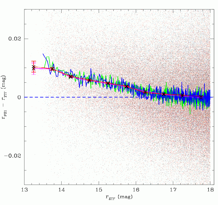
Magnitude Bias
The initial results suggested that the bright-end magnitude bias within a field (shown above) is consistent for a given quadrant, but varies between each of the 64 CCD quadrants and filters. This seems most likely a detector gain issue. In discussions with R. Smith, he mentioned that the detector gain had been found to actually be significantly non-linear. There was also suggestions of the so called brighter-fatter effect and other detector-based possibilities.
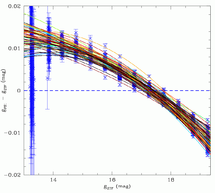
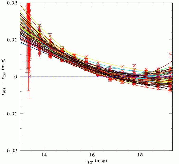
Fits to the ZTF vs PS1 magnitude bias.
Left: The fits to the g-band magnitude bias for each quadrant.
Right: Fits to the r-band magnitude bias for each quadrant.
When the photometry was combined the magnitude bias was found to extend to faint magnitudes. So the full photometry data sets were extracted for the selected fields (total 12 million sources). However, at the faint end, the magnitude bias becomes dominated by an Eddington bias. Thus the magnitude bias was only fit for ZTF sources brighter than ~19.25 to avoid this. For each quadrant, quadratic fits were used since the bias was evidently not linear.
Conclusion:
To properly calibrate ZTF magnitudes to PS1, all ZTF photometry
needs to corrected for the clear magnitude bias.
Questions:
What is the exact origin of this bias?
Is it safe to assume the fits to bias are
OK at magnitudes fainter than 19.25?
Is there a way of verifying this?
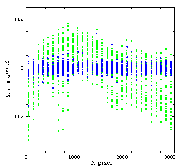
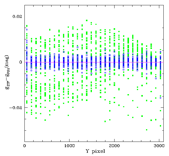
Spatial Structure within ZTF Photometry
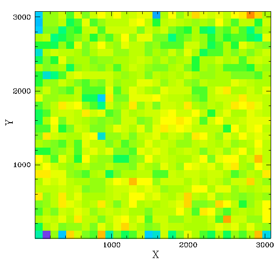
After correcting for the magnitude bias it was clear that the spatial variations in photometric uncertainty within a quadrant (above) were a reflection of the spatial variations in the photometry.
Corrections for this internal residual structure were underway by the Desy group using starflats. That is, observations where a single field(?) is dithered and photometry of sources are remeasured to determine spatial variations. The combined and binned starflat data is shown above. Since this data is taken in sequence on a single night, very similar observing conditions are expected. Thus the result should be largely free of effects due to changes in observing conditions.
A clear way to check the starflat-based determination of the spatial systematics is to use the photometry itself. The advantage of this data is that there are far larger numbers of measurements can be used in the determination. In principal such a dataset could have hundreds of times the amount of photometry in the starflats. Such a large data set makes it possible to limit the selection to the bright stars that have smaller intrinsic uncertainties than the systematics. So, overall the spatial variations can in principal be better sampled since millions of bright sources can be used to determine the structure within each of the 64 quadrants. However, in contrast to starflats, more careful consideration is needed to address any possible biases due to real variations observing conditions.
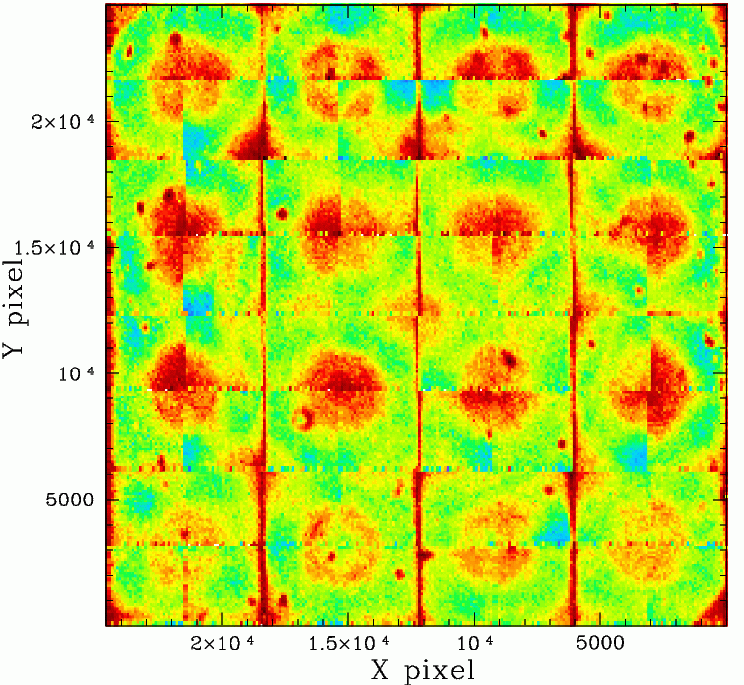
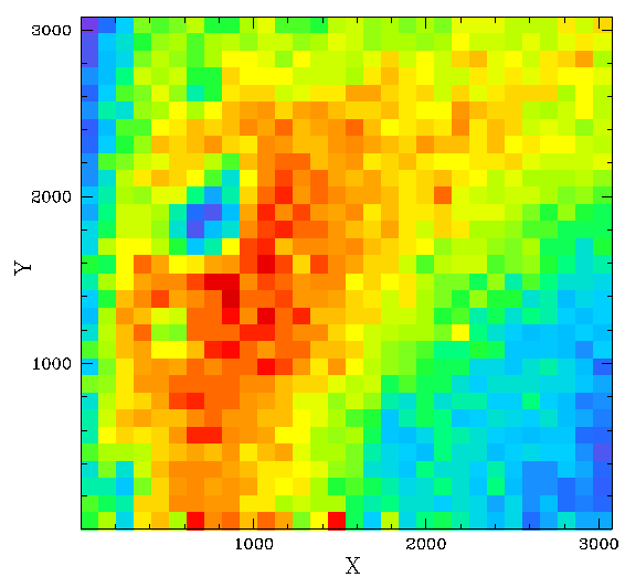
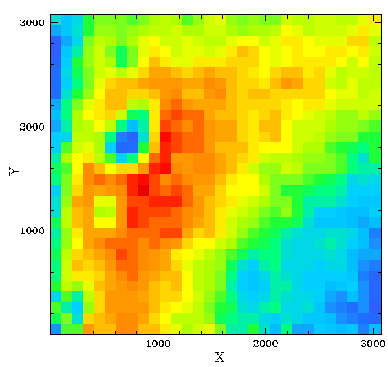
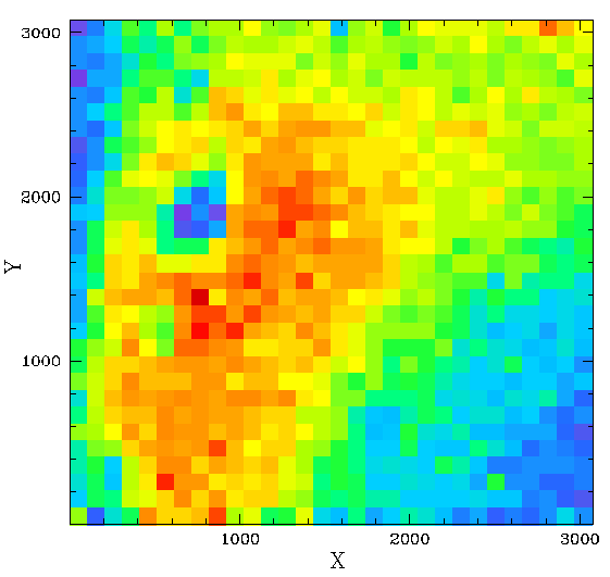
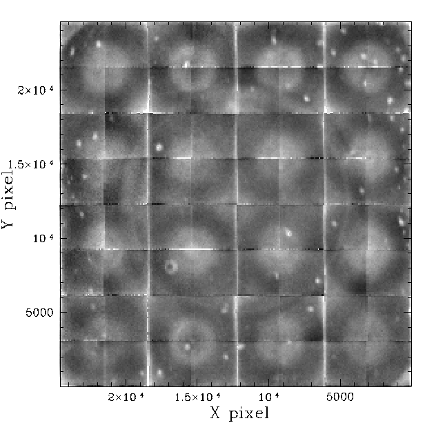
Desy Group full Camera FoV G-band systematics from starflat data
matched to PS1. Left: the structure found with the starflat analysis
Right: the residual structure after correcting with starflats.
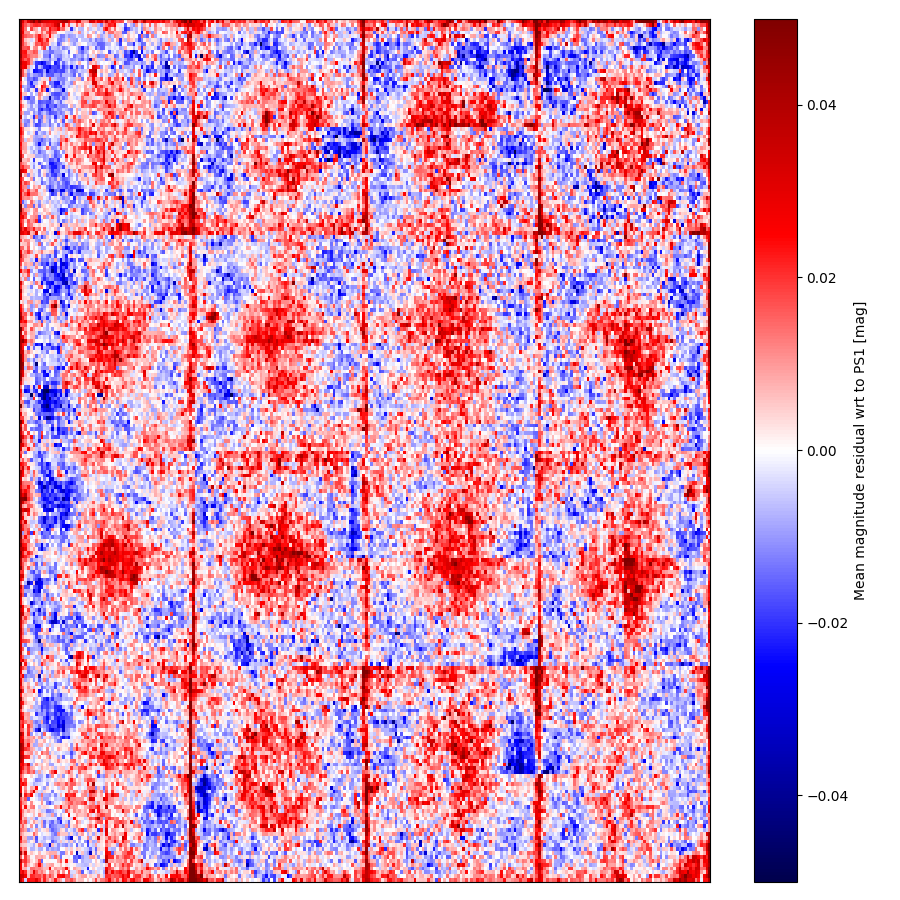
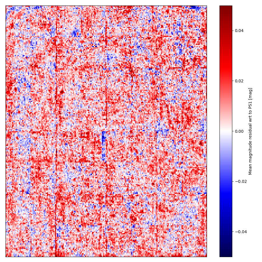
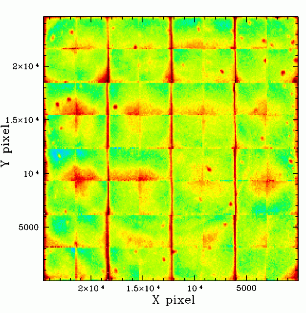
Full Camera FoV g-band systematics based on photometry data matched to PS1 (c.f. left figure above). Colours range from ~-0.03 to 0.03 mags.
Comparing the systematics from starflat data and those from combined photometry we see that the general structure of the systematic is this same. However, the structure based on the photometry is smoother and clearer due to the higher S/N of this combined photometry results.
Strong structure is seen on edges (due to reflections and possibly charge transfer issues seen in other data?) and discrete lumps (due to dust). Full ccd show large features that also visible in the flat fields. Suggesting possible problems with them.
Notably, the borders of the CCD quadrants exhibit discontinuities between quadrants. This is most likely due to gradients spanning the full CCDs. Since the data is calibrated at the quadrant level this introduces an offset at the borders. This suggests that structures spanning full CCDs cannot be fit without correcting this.
The corrected starflat data still exhibits some clear spatial structure that is like hard to remove with with either data set.
Fitting the spatial structure
The extent of the structure within individual quadrants is very significant and most likely due to problems with flatfielding and gain corrections. That is to say, systematic uncertainties in the flatfields are propagated into the data and become apparent when the data is combined. This effect may be increased by the fact that different flatfields are constructed and used each night even when no changes have been made to the telescope setup.
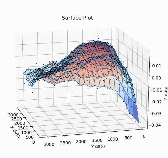
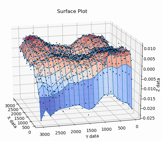
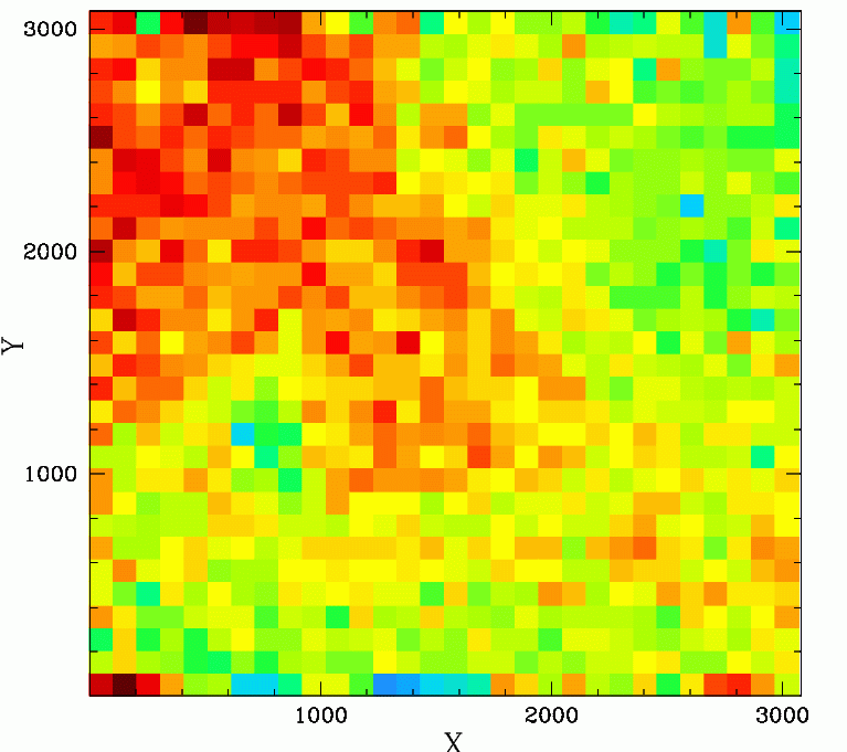
Surface plots of the binned spatial distribution of magnitude
residuals wrt PS1 for two quadrants. Left: the residuals for CCD 16,
quadrant 1, zg. Right: the residuals for CCD 16, quadrant 4, zr.
Z is the magnitude offset and X and Y are the CCD coordinates.
Attempts to automatically model the photometric residual surfaces were undertaken with numerous (~100) different types functional fits. These ultimately failed to produce satisfactory results since the dust artifacts and very strong edge effects produce abrupt deviations that is not well modeled by smooth functional fits. Fitting in multiple steps is also not ideal.
G-band magnitude residuals wrt PS1 before and
after correcting for structure with the quadrant.
The green is the original binned data and the blue are
the residuals after subtracting the spline fit.
Attempts to fit splines to the unbinned data were also unsatisfactory (residuals > 0.005 mags, clear systematic variations and spikes) because the raw data was insufficiently constrained. However, since the wasn't any clear significant structure on scales less than a couple of hundred pixels the binned data was used. If localized structure is actually present (that is not accounted for by flatfields, etc), corrections will require far more photometry (than ten fields) to properly constrain it.
As shown in the figure above, quadratic B-spline fits of high order (440 knots) were used to fit the binned data give good fit residuals (sigma of 0.002) magnitudes without spikes due to poor constraint. Although, care is still required to check the fits on image edges where strong gradients are present.
ZTF magnitude residuals relative to PS1.
Left: The residuals from data combine from nine fields within
the same band, CCD, quadrant (ccd 5, quadrant 1, g-band).
Middle: the spline fit model for the data.
Right: the residual after subtracting the spline fit.
Colours range from ~-0.03 to 0.03 mags.
The figures above show how well the spline fits represent the actual structure in the binned photometry.
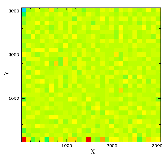
Verifying the spatial structure corrections.
In order to verify that the corrections determined with the original photometry data set work for other fields work for both the selected data and other data in general it is necessary to verify the analysis. To do this, for a few quadrants, I selected an additional set of photometry for 8 fields. This photometry was corrected for the magnitude bias and quadrant structure.
Residuals for fields not in the original calibration.
Left: Systematic differences between ZTF and PS1 for g-band
photometry in CCD 05 Quadrant 1.
Right: Photometry minus the spline fit for the new fields.
The sigma of corrected residuals wrt PS1 (for sources with g < 17.5), for both the original set and the new ones, is ~0.008 mags. This suggests that the same structure is seen in multiple fields with a very similar in amplitude and distribution. That is to say, the result from the combined photometry is not strongly affected by variations in the observing conditions. However, see more analysis below.
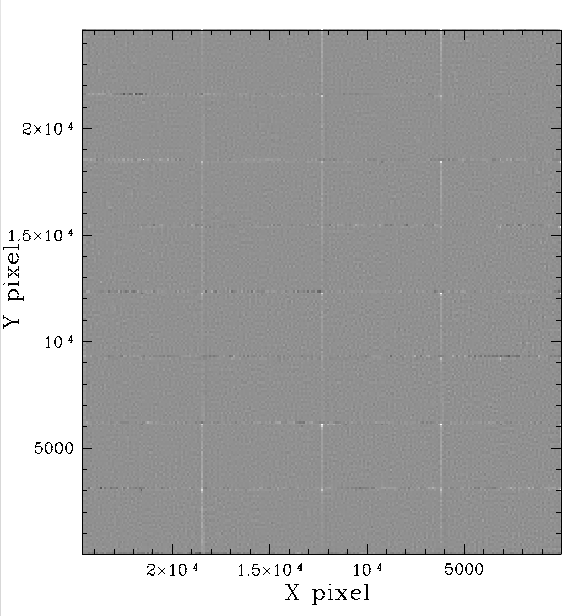
Correcting structure across the full ZTF FoV
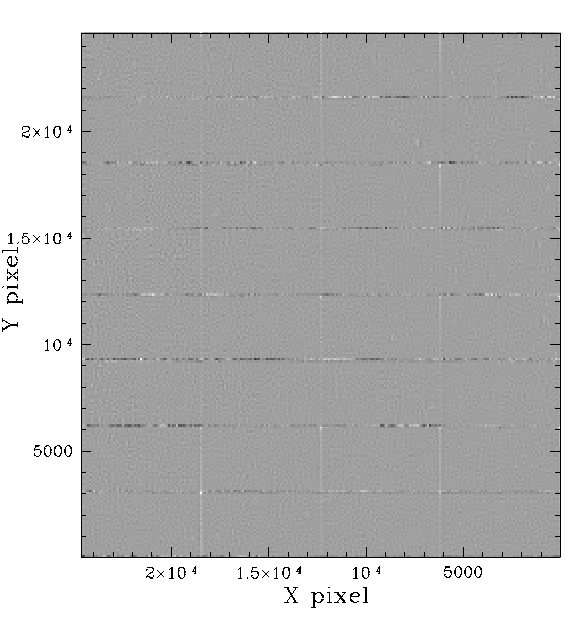
Initial fits to the structure were poorly constrained on edges where few sources are detected. This is due to significant variations in pointing between the reference frames and the individual observations. To improve this situation the photometry sample was increased by a factor of three (so that each quadrant contained photometry from ~30 fields). The resulting residuals were much more clearly defined (c.f. the figures above). The residuals from the binned residuals spline fits were reduced from two milli-mags to one for many fields. Nevertheless, accurate values of residuals on quadrant edges was still not as good as it could be in many cases. Thus, extra care was taken to fit the individual quadrant values by hand. The edge bins with few points were further constrained by adding additional faint sources and by interpolating the values from neighbouring bins.
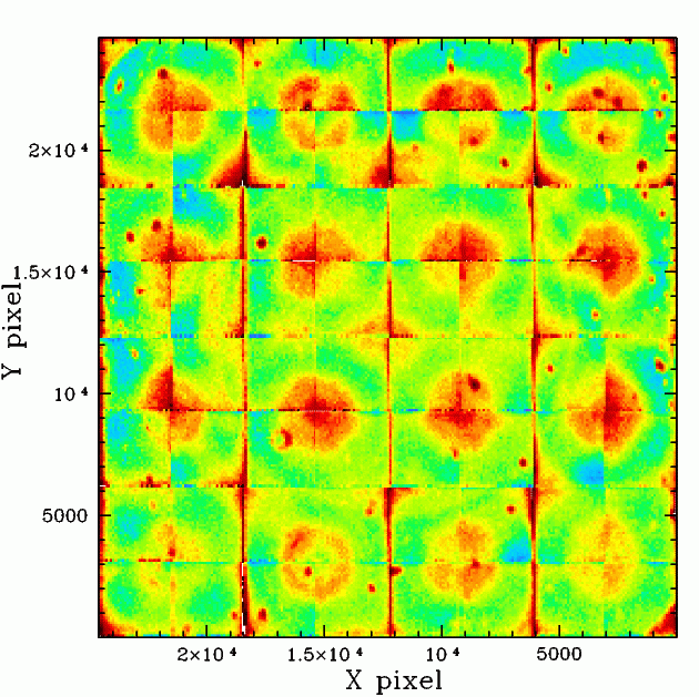
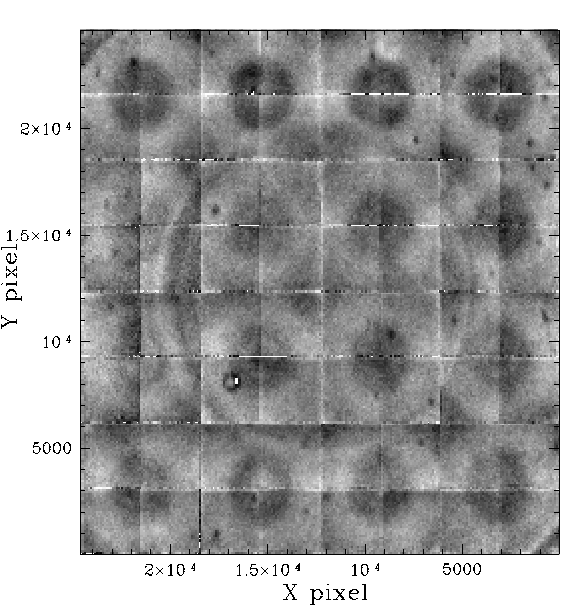
The g and r-band ZTF magnitude residuals wrt
PS1 based on combining the photometry from ~30 well sampled
fields in each quadrant.
With the higher S/N of the new combined data some evidence of a large ring is seen that is due to the focal plane pattern. This is what was initially expected from the starflat analysis since it is seen in the DES analysis (Berstein et al. 2018, PASP, 130, Figure 2).
Since rainbow colour maps can exaggerate the presence of structure, additional greyscale images of the same data are given below. However, the variations at the edges of adjacent quadrant becomes less clear in the grayscale images since these differences are slight.
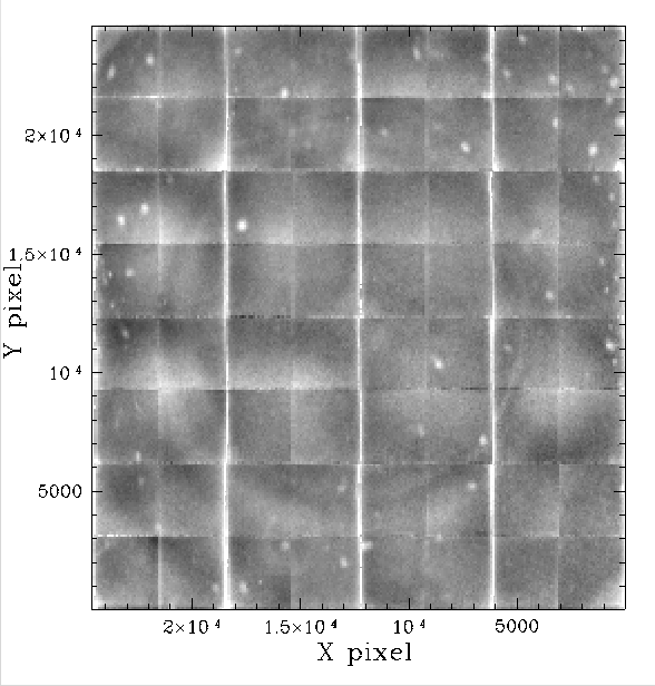
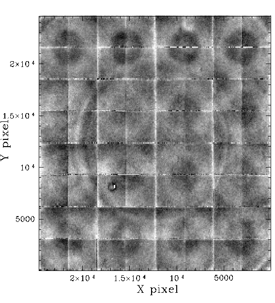
The g and r-band magnitudes residuals wrt PS1.
As above but with a continous grayscale colour map to show.
The structure within g and r-bands is very similar with only slight differences in residual amplitude and a few dust spots. This suggests that most of the dust spots are not on the filters, but other optics.
The g and r band magnitudes residuals
after subtracting the spline fits to each quadrant.
After fitting the spatial structure in each quadrant and subtracting it, the residual photometric structure is given above. The g-band data has more significant residuals at the top and bottom of quadrants than r-band due to the higher amplitude of differences compared to PS1 data. The amplitude of the residuals of the left and right edges of CCDs and similar in each band.
After applying the corrections to ~3 million sources with 14 < mag < 16.5 from across the full FoV we find residuals of ~7 milli-mags. Thus, overall the uncertainties are generally expected to be less than 1 percent.
The corrected data does exhibit extended tails (compared to a Gaussian fit) due to the remaining edge effects. Hence objects falling near edges will generally be more uncertain. The same edge structure is seen in DES skyflat subtracted residuals. We note that few objects are expect on the edges since such sources were clearly absent from the data.
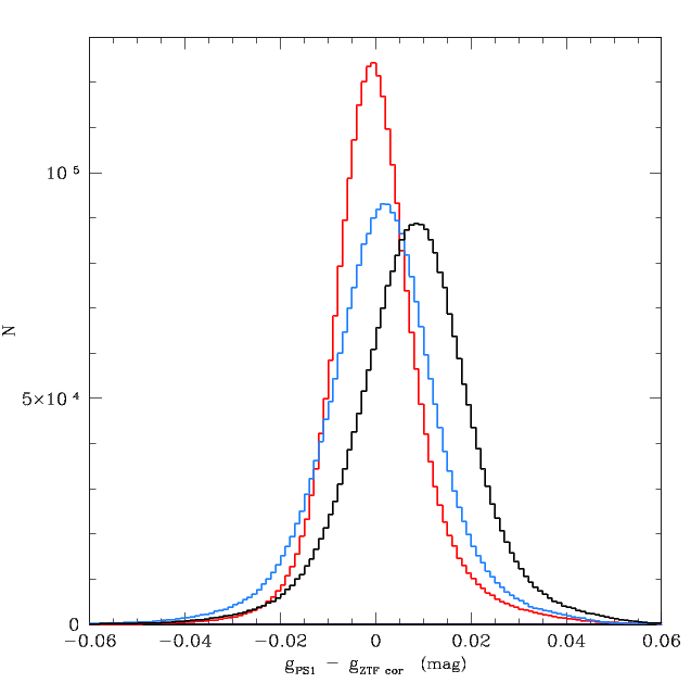
The residuals for ZTF g-band wrt PS1. Black histogram original ZTF photometry calibrated to PS1 for ~3 million source with 14.0 < g < 16.5 . Blue, the histogram after applying the magnitude corrections. Red, the result after applying magntiude and structure corrections.
Conclusions:
The ZTF data exhibits significant structure within CCD quadrants
that can cause offsets of up to ~0.04 mags on the edges and at
the locations of large dust spots. These features can be corrected
to a high degree of accurary. Correcting for these features by
fitting the structure brings the photometry into agreement with
PS1 to better than 1%.
The colour dependence of photometric residuals
During discussions of correcting the residual structure using photometry or starflats there was mention of the possible colour dependence of the structure. To quantify this more clearly I compared the residuals wrt PS1 in g-band with those in r-band.
The difference between ZTF g and r-band residuals compared to PS1 (CCD 5, quadrant 1).
This figure shows that the structure within a quadrant varies significantly between g and r bands. This figure relates to the same quadrant shown above. Based on the structure within that data we see that the difference between g and r is very likely not simply an offset or scaling between the two bands.
A difference in the g and r-band residual structure implies that there is some spatial variation in the colour response (in addition to possible local differences such as dust spots on filters). Significant difference are expected due to the AR coatings that vary between rows of CCDs and apparently even between individual CCDs. However, such differences are not expected on smaller scales.
Colour dependence across the full FoV
With the large sample of ZTF photometry used to determine the spatial structure, we investigate the differences between the structure in the g and r-band observations.
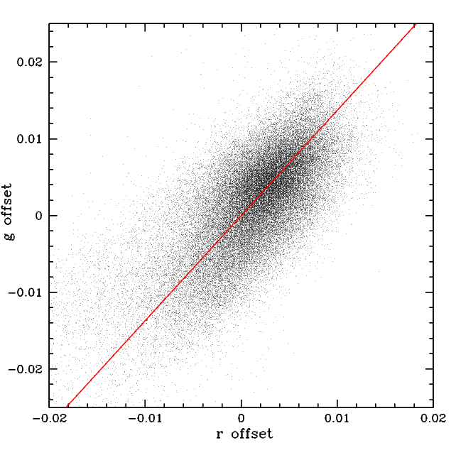
Comparison of g and r-band residuals. The red line has slope 1.37 corresponding the average ratio of g to r-band residuals.
Comparing the values in each of the g and r bins we see the the g-band residual structure is approximately 37% larger than the r-band structure. Notably the bulk of the residuals are not centered on zero, but near 0.005 mags in g and r.
The difference in structure between g and r-band data. The
left plot is the residuals in g bins minus those in r. In
the right plot the differences in residuals after scaling
the r-band values by a factor on 1.37 (to account for the
amplitude difference noted above).
If we subtract the binned r-band values from those in g we see that that the vertical lines on the edges of CCDs largely disappear, while the dust dot-like features remain. This suggests that the edge effects themselves are not wavelength dependent while the affect of the dust spots is.
To confirm this we multiple the r-band structure by 1.37 (to account for the difference in average offset amplitude) and subtract this from the g-band data we that the dust spot disappear. This suggests that the dust spots follow the same trend as the overall amplitude difference (i.e. they have the same dependency). However, large structures that are centered on each CCD remain. This suggests that the residuals cannot be account for by purely scaling the results between bands. The central and outer circular features of the focal plane become clearer in these figures.
Conclusions:
The source of this colour dependence of the observed photometric offsets
is most likely variations in sensitivity that are not being taken into
account by the flatfields. The lack of clear trend covering the
whole focal plane suggests that differences in the offsets between
g and r-band are not due to large scale problems, such as non-uniformity
of the filters (i.e. filters coatings not going to the edge).
However, this may still be present at a low level.
The lines along the edges of CCDs have equal amplitude in g and r-band suggesting that the effect is not wavelength dependent. This suggest the affect originates from behind the filter (these have been noted as scattering from CCD frames). In contrast, most of the dust spots exhibit the same scaling as the general background structure and do not vary between filters. The dots are thus generally not located on the filters. A small number of out-of-focus rings are seen in only one filter suggesting these are on the filter itself. The overall circular structure and spots within each CCD exhibit exactly the same pattern present in each combined flatfield. This suggests that there are errors in flatfielding. Significant variations in the flats over time are present. So this is of no surprise.
Whatever the cause of the colour dependencies, corrections are required for both g and r separately. Some consideration of how these offsets affect objects of varying colours differently is worthwhile. This effect is equally important regardless of whether starflats or combined photometry is used for spatial corrections.