| Topics |
|---|
| Time dependent flatfield variations. |
| Flatfield systematics all quadrants. |
| Flatfield colour variation effects. |
| Average flatfield colour response. |
| Combined flats from indivudal CCDs. |
| Temporal variations in flatfields. |
| Variations due to Cleaning. |
| The effect of Hexapod location. |
Structure in ZTF flats.
Variations in flatfields can tell us about changes in the throughput of the optical and electronic systems. Large variations over a short period can tell us when there are significant problems. Smaller trends can us about the regular degradation due to dust or low-level degradation of the electronics (such as variations of the LEDs). For example, R. Smith suggested that we can tell how often cleaning of optical elements are required by looking at variations in flatfield levels.In order to determine this IPAC (F. Masci) provided values of flatfield medians for all nights. I averaged over multiple different LED lamp exposures for each night in order to increase the S/N.
To roughly determine how flatfield values might vary across the ZTF camera I selected one quadrant in each corner of the camera as well as two near the center.
Combined nightly median flatfield g-band values. The left figure shows the values for CCD_quad combinations 1_1, 4_1, 7_1 and 6_2. The right figure for quadrants 13_1 and 16_1. Note: slight offsets have been applied for display purposes.
From the figure above we see that there is significant structure in addition to the general decline expected due to accumulating dust. The right panel of the figure shows that there are extinction events that affect the upper region CCDs far more than the lower ones (changes as much as 10%). Individual traces are actually combined from multiple exposures of separate LEDs. Unfortunately, the origins of each exposure was not unambiguously marked within the metadata (the number and order changed over time).
The causes of the events shown in the are not all known (to me).
Some known and possible causes are summarized as fellows:
| Feature | Date | Source |
|---|---|---|
| A | June 26 2018 | Change to gain levels? |
| B | July 18 2018 | Cleaning followed by thick (oil?) deposit(?) |
| C | Aug 28 2018 | Throughput increase due to gain change(?) |
| D | Oct 9 2018 | Camera removed. CCD gain change(?) |
| E | Jan 5 2019 | Linearity change(?) |
| F | Oct 22 2019 | CCD gain levels changed. |
| G | Dec 10 2019 | Cleaning performed. |
Based on ~290 day span between E and F (which is free of significant
external changes) the
decline in throughput due to dust is 0.011%
per day (~1% per 3 months).
Flatfield systematics for all readout channels.
All ZTF science images are processed by using multiple LED lamps that are combined to produce flatfields. Thus, the most accurate calibration of ZTF photometry requires accurate flats and an understanding of events that affect the throughput.In order to investigate how the events noted above (A-G) vary between CCD quadrants I determined averages for all quadrants. Values averaged over all epochs were then subtracted for each quadrant. To account for variations across the focal plane (normalized versions of these variations were also investigated) we investigate quadrants separately.
Below we plot the averaged g,r and i-band flatfield counts over the span of regular ZTF observations. The white areas are times when no flatfield data was taken (e.g. camera removed).
Variations in flatfield count levels over the period of ZTF observations for g,r and i-band filters (top to bottom). In each case the full range of colours (dark red to dark blue) represent a ~10% change in throughput.
As with the line plots at the top we can see that there are large variations due possible camera warming events. This event apparently mainly led to deposition of material (oil?) on the upper row of CCDs (RCs 48-63). This led to a decrease in throughput of ~10%. The variations in g and r-band due to this appear similar. The i-band variation may be less significant. However, the i-band data is generally noisy.
From the figures we can also see a few individual sets (nights) of flatfields are clearly outliers. These tend to lie below the general declining trend. It is not yet clear whether these flats have be used for the processing. If so, they are likely to have caused photometric outliers since there are almost certainly intra-quadrant variations (unless these events were really CCD gain changes?) while the calibrations themselves are only performed on full quadrant levels. Additionally, the decline due to the deposition event C (starting ~220 days) clearly increases with time and is very likely to affect photometry from the upper row CCDs. Likewise, event D (~320 days) mainly affects the same CCDs, in a similar way. The cause of this event is currently unknown. In contrast event A (~195 days) appears to affect all CCDs to a similar levels. This may have been a gain change since the saturation levels in the corresponding images are lower.
Additional outliers are seen in g and r-band for RCs 0-25 from days ~100 to 110. If these flats were used in processing, they likely to have affected much of the early ZTF photometry in those CCDs. However, there is a possiblity that these are artifacts in the data due to changes in the number of LED frames used (and thus the combined average).
Flatfield colour evolution.
In order to investigate the how events such as waveform/gain changes and vacuum loss deposition events might of affected photometry I decided to look at how the colour throughput changes with time. This is investigated by using the ratios of flatfield median values for each quadrant.
Ratio of g-band to r-band flatfield fluxes as a function of time and CCD quadrant.
In the figure above we see significant differences in the ratio of g to r-band median counts between quadrants (mainly between CCD rows in general). The central two rows of CCDs are different than the outer ones due to the presence of an AR coating. Over time slight changes in these ratios can be seen. These large variations between rows are likely a combination of varying CCD sensitivity, filter throughput and possibily some large scale flatfield illumination differences.
Variation in the ratio of g to r-band flatfield median fluxes relative to the quadrant average as a function of time.
To better see the temporal variations, the average colour for each quadrant was subtracted as shown above. The results suggest that variations in the overall colour response are less than 2%. The long timescale trend over time is likely related to dust build up seen image plots above. This suggests that the dust exhibits a significant wavelength dependent aborption (possibly a Rayleigh scattering dependence). Significant low level structure is seen superimpossed on the overall changes. The reasons for these changes are not clear. There may be issues related to temperature variations of the LEDs and optics.
Interestingly, the deposition events that were clearly seen in the upper row of CCDs in the figures above, are not very clear here. This suggest that the material deposited in the heating events probably has very little absorption wavelength dependence (in the g to r range), or that they were actually gain changes.
Average colour response
The ratio of g to r-band flatfield median fluxes averaged over all current data. Left and right are the same except for the colour maps.
To better understand the colour response of the camera, here I have plotted the average g/r flatfield flux ratios across the focal plane. Since all CCDs are illuminated simulaneously and hopefully evenly, differences between ratios should reflect real variations in the overall (optical + electronic) colour response. Intra-CCD variations are clearly smaller (< 1%) than inter-CCD ones (~9%) and should reflect variations in the electronics and reflective coatings.
Notably CCDs 11 and 12 perform differently than adjacent CCDs. CCD 11 has previously been noted to have better throughput (fainter ZPs) than other cameras. CCD 12 has previously been found to give poor results in i-band starflats and may have issues.
The middle two rows of CCDs are offset from the top and bottom rows due to difference in the AR coating. Quadrant level variations in filter-based throughput (such as due to coating variation) as a function of location are not obvious. Nevertheless, assuming the overall colour variations are real, than the colour coefficients of our calibrated photometry should vary systematically between quadrants (readout channels).
Combined Flats for individual CCDs
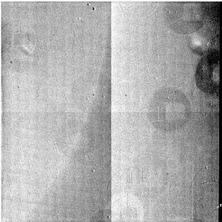
To investigate the structure within the flats of individual CCDs I simply combined the data from each of the four quadrants into a single image without any scaling. I plot these alongside the binned residual photometric structure determined earlier.
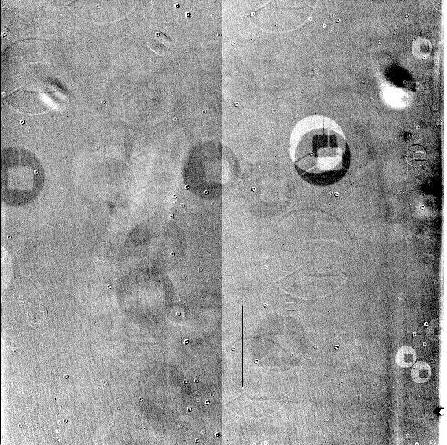
The combined g-band flatfield from 2020-02-27 for CCD 13 compared with the binned residual photometry structure (right).
The combined g-band flatfield from 2019-12-18 for CCD 14 compared with the binned residual photometry structure (right).
The structure within the combined flats very closely matches that seen in the residual photometric spatial structure. This structure includes both dust spots and the offsets seen at the borders between readout channels within the CCDs. This result adds additional weight to the conclusion that a significant source of the residual spatial structure in ZTF photometry is imperfect flatfielding.
Ideally the combined flatfields for individual CCDs should be continuous. However, difference at edges of a few percent are clearly seen. The source of the border features could possibly be due to the flatfield normalization being undertaken on a per quadrant basis (as communicated by F. Masci). Some difference may also come from difference readout gains between channels.
The average differences are expected to be small and appear consistent with the variations in intra-CCD flatfield median values given above. Interestingly, in each case investigated, quadrants 1 and 2 exhibit some additional low-frequency spatial structure that varies from that present within quadrants 3 and 4.
Temporal Variations in ZTF Flatfields
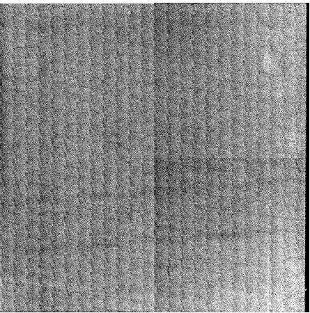
To see the scale and extent of spatial variations in flatfields over time I combined set of flatfields taken on a number of dates. Flatfields taken between 2019-01-05 and 2019-10-22 are consider good since their median values only exhibit a continuous decline due to dust accumulation (see above). I selected the combined flatfields from CCD 5 taken on 2019-02-01 as a reference set since these were near the beginning of this period and had no obvious issues. Each of the other combined flatfields was then divided by this reference flatfield.The resulting flatfield ratio images for each date are shown below.
Binned variations in combined g-band flatfields for CCD 5 relative to reference date (2019-02-01). Left: 8 by 8 binned ratio image for 20180407. Right: 8 by 8 binned ratio image for 20180607.
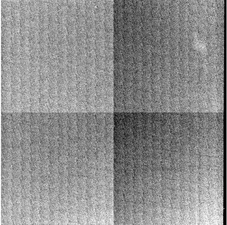
As above. Left: ratio image for 20180807. Right: ratio 20181007.
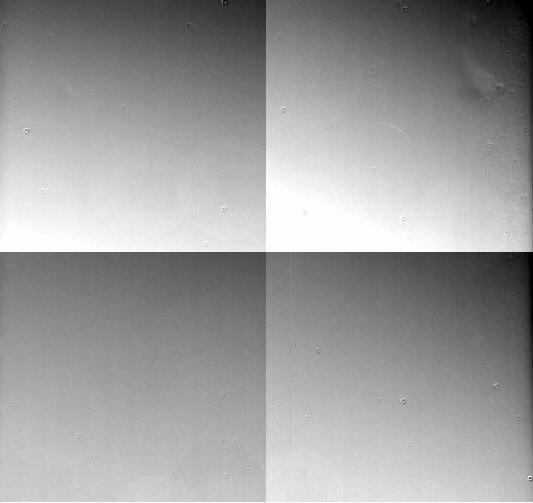
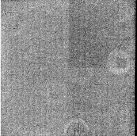
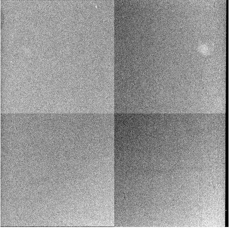
As above. Left: ratio image for 20181215. Right: ratio for 20190110.
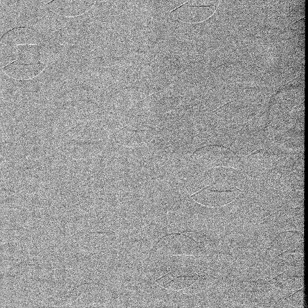
As above. Left: ratio image for 20190131. Right: ratio for 20190210.
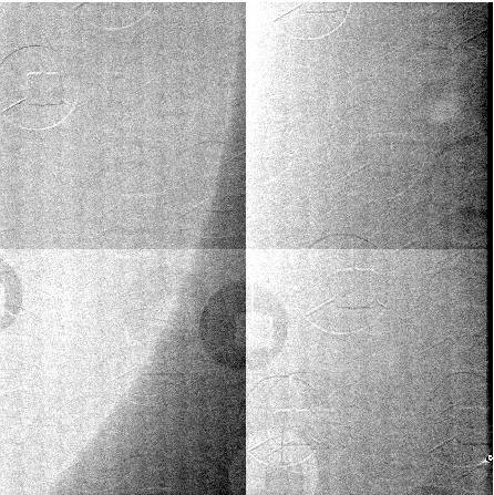
As above. Left: ratio for 20190407. Right: ratio 20190607.
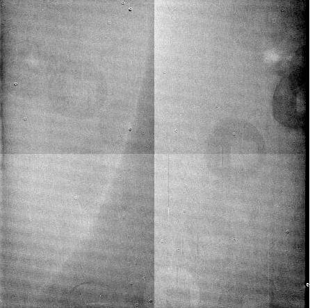
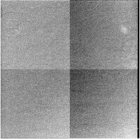
As above. Left: Ratio image for 20190821. Right: ratio for 20190907.
As above. Left: ratio image for 20191007. Right: ratio image for 20200115.
An expectation for these ratio images is that, if flatfields are stable over time, the images should show very little spatial structure. Generally the ratio images should simply scale with the variations in the flatfield median values. Indeed, this is what we observe for the flats taken near the reference date (for example see the ratio image for 20190131 above). Nevertheless, some variations in the structure are expected if new dustspots appear or are removed during cleaning. What we see is that some of the large discrete constant features (due to dust spots and reflections) vary over time. In some cases there are large differences in the flatfield gradient (for example see 20181215), and often there are significant variations in the values on right edge for this CCD.
The wide range of varying features seen within the flat ratio images clearly shows that the flats are not stable over the span of observations and thus not simply the scaling of a single underlying illumination pattern.
The Scale of Flatfield Variations
To determine the extent of the spatiotemporal variations I determined the range of values for each of the ratio images. For each distribution I determine the amplitude of variation after clipping a small (~1%) number of pixel values from the upper and low tails of each distribution.Below I plot the amplitude of variation for each of the ratio images above.
Values of the amplitude (range) of variations between flatfields and the reference. The "good data" range are for images taken between Jan 5 2019 and Oct 22 2019 (the region denoted E to F above). The red point marks the date of the reference frame.
Considering the period of "good data", we see that flats taken close to the reference flatfield (red point) exhibit very low amplitude (< 0.2%). These differences gradually increase over time to ~1.5%. The differences between the reference image and earlier images (when a number of discrete changes are seen in the flatfield medians) is 1.5 to 2.5%.
The photometry used to determine spatial residuals was taken during the period from around March 2018 to June 2019. Thus, it is of little surprise that similar the major spatial variations in flatfields also appear within the photometry. Nevertheless, the amplitude of the flatfield variations does appear to be smaller than the scale of the photometric residual structure. This suggests that additional factors are also at play. For example, photometric errors due to spatial variations in the PSF shape could increase the observed photometric residuals.
Additionally, some fraction of the spatial variations seen in the flatfields are undoubtedly real. Therefore, we should expect that the flatfield variations will have a smaller observed affect on photometry. Nevertheless, unless they are very accurately characterised, the presence of significant abruptly varying flatfield structures will lead to inaccuracies in the flatfields that propagate to the photometry.
The Effect of Cleaning
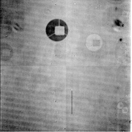
The cleaning on 2019-12-10 resulted in a 4% increase in throughput. To determine the effect of cleaning on the spatial structure with the flats (e.g. whether the dust caused increased scattering), I took the ratio of a number of post-cleaning images to that a couple of days before cleaning (2019-12-08).
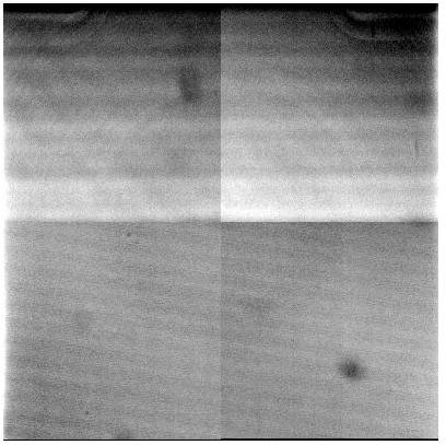
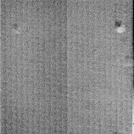
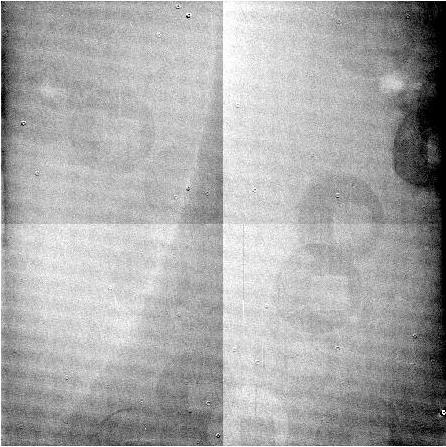
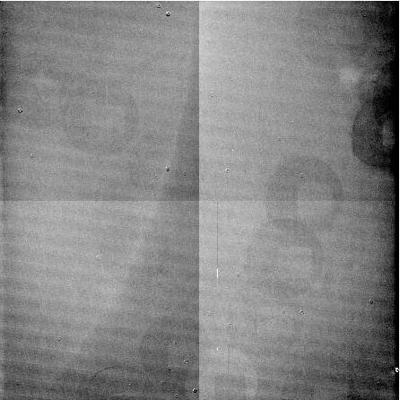
Ratio of CCD-5 flats before and after cleaning (binned 8x8). Left: the ratio of the flat from 2019-12-11 to 2019-12-08. Right: the ratio of 2019-12-12 to 2019-12-08.
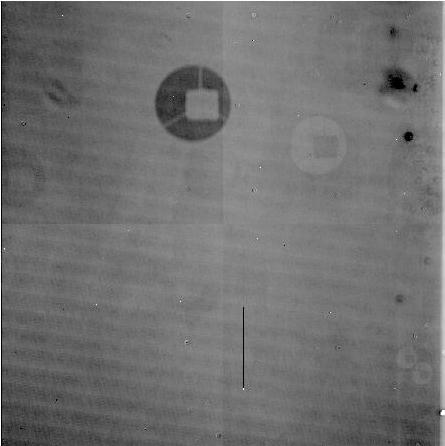
Ratio of CCD 5 flats before and after cleaning. Left: the ratio of the flat from 2020-01-14 to 2019-12-08. Right: the ratio of 2020-01-15 to 2019-12-08.
From the resulting images we see is gradients across the quadrants suggesting that clean the corrector has a non-uniform effect on the flatfielding. However, this effect is only 0.1%. Since the effect is so small it is hard to determine whether this is due to the cleaning or some other effect. However, it is unlikely to be due to a gain change since that only creates an offset which is removed during normalization.
The cause of the vertical banding in the ratio images from 2019-12-11 and 2019-12-12 is unknown, but is possibly related to interference changing at the time of cleaning. However, as the amplitude of this effect is < 0.01% it will not be followed.
The change in the dust spot in the upper right is < 0.03% while the spot at this location cause a 6% effect. Thus the occurance is not due to a significant change (such as a removed spot).
As with the images above there is a dark line along the right edge (with width ~70 pixels). These areas only represent a 0 to 0.2% gradient and are thus exagerated at this scaling.
The ratio of the post-cleaning flats show the faint presence of large streaks across the images (very slightly below 1.0). This suggests that the cleaning itself may have introduced these features. The features are much less significant than the change in background gradient.
To better quantify the main trends within the ratio images I averaged the y pixel (columns) values across the lower two quadrants. I then did the same for the upper two quadrants.
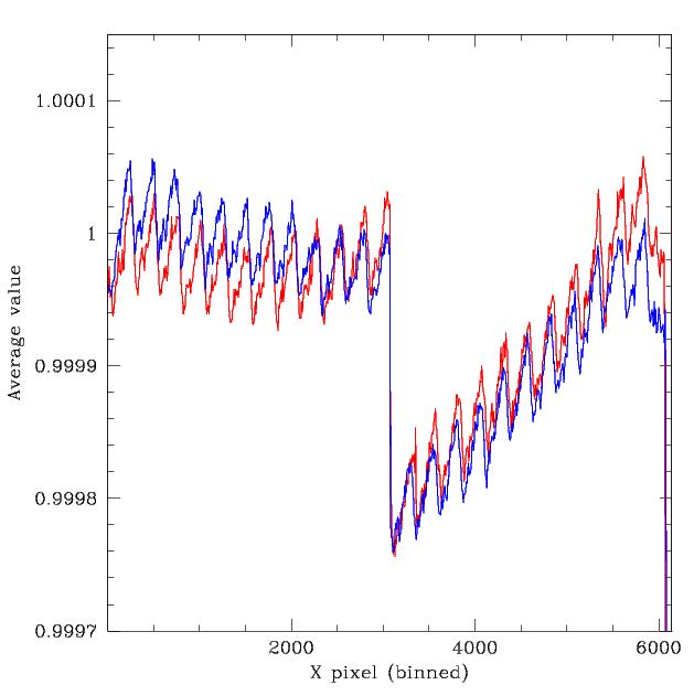
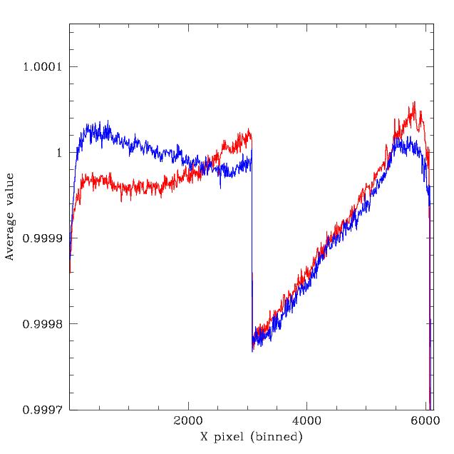
Average values of ratio of CCD-5 flats before and after cleaning (from images binned 8x8). Left: the ratio of the flat from 2019-12-12 to 2019-12-08 for the lower two image quadrants (3 & 4) red line and the upper two quadrants (1 & 2) blue line. Right: Same as left but the ratio of 2020-01-14 to 2019-12-08.
The plots above show a clear gradient trend in the flatfield ratios. The amplitude of the gradient is very small here (~0.02%). However, this is actually much smaller than the true gradient since we have averaged over the quadrant and the gradient actually runs diagonally rather than horizontally. The banding structure becomes even clearer in the averaged data. The level of variation here is not large enough to significantly affect the photometry. The discontinuities at the borders edges of quadrants are also very clear as well and along the CCD edges. The ~0.2% variation on the right edge of CCD-5 is large enough to affect the photometry slightly. This will also be the case for other CCDs, but will occur on different edges.
The Effect of Hexapod Location on Flats
During a calibration meeting there was a suggestions that the location of the Hexapod during flatfield might not match typical ZTF observations. This could produce a slightly different illumination pattern in the flats.On 2020-02-11 the Hexapod position was set to zenith to better match observations. To determined the effect of this I have taken ratios of flats with the change to those before.
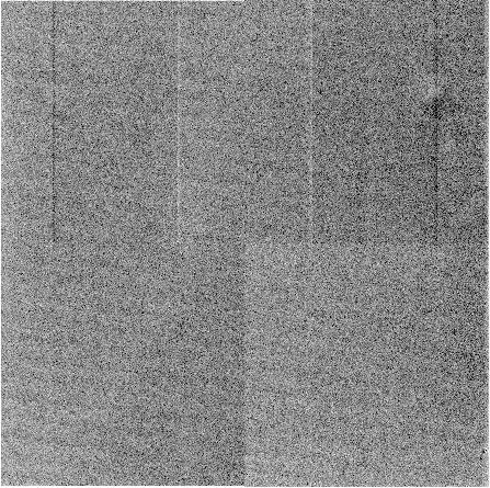
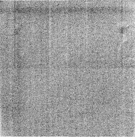
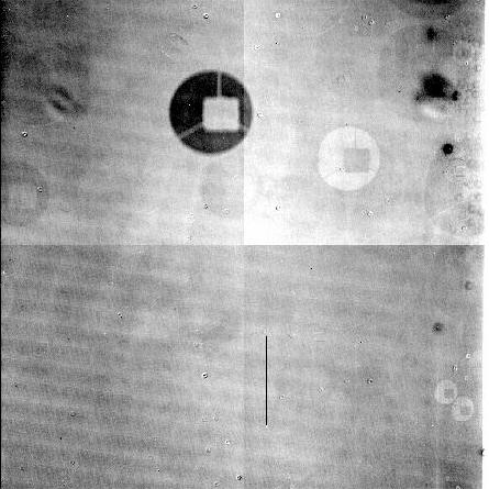
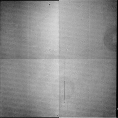
The 8x8 binned flatfield ratio images for CCD 5, g-band. Left: the ratio of two nights (2020-02-09 and 2020-02-10) before the change. Right: the ratio of the night after the change to that before it (2020-02-11 and 2020-02-10).
The amplitude of this difference between flats taken on 2020-02-11 and 2020-02-10 is ~0.1%. Similarly the ratio of 2020-02-09 to 2020-02-10 is ~0.1%. This suggests that the location of hexapod has little effect on the flatfielding. Nevertheless, the ratio images do suggest that there is a small affect. There are dark bands near the top and left sides of the image containing observations from 2020-02-11.