| Topics |
|---|
| Motivation for using Zubercal. |
| Initial Zubercal tests. |
| Improving the Zuber calibration. |
| Correlations of physical observables. |
| Inclusion of PSF-based parameters. |
| Atmospheric Transparency. |
| The Importance of Transparancy Changes. |
| A Broader Investigation of Transparancy Variations. |
| Nightly Photometric Variations. |
| Correcting photometry for Transparancy Variations. |
Motivation for Ubercalibration of ZTF photometry
The current photometric calibration of ZTF is based on the comparison of each individual quadrant image with a set of calibration stars selected from PS1 DR1 for each quadrant. These PS1 stars have been ubercalibrated with photometry noted to be good to approx 1% and are selected within a colour, magnitude and density (crowding) range as noted in the ZSDS. However, due to the differing stellar density and reddening properties of ZTF fields, the result of these selections is that a different population of calibrators used in different fields. This in turn results in substantial variations in the accuracy of the zero points and colour calibrations. Principally, the lack of available calibration stars limits the resulting accuracy of the calibration.
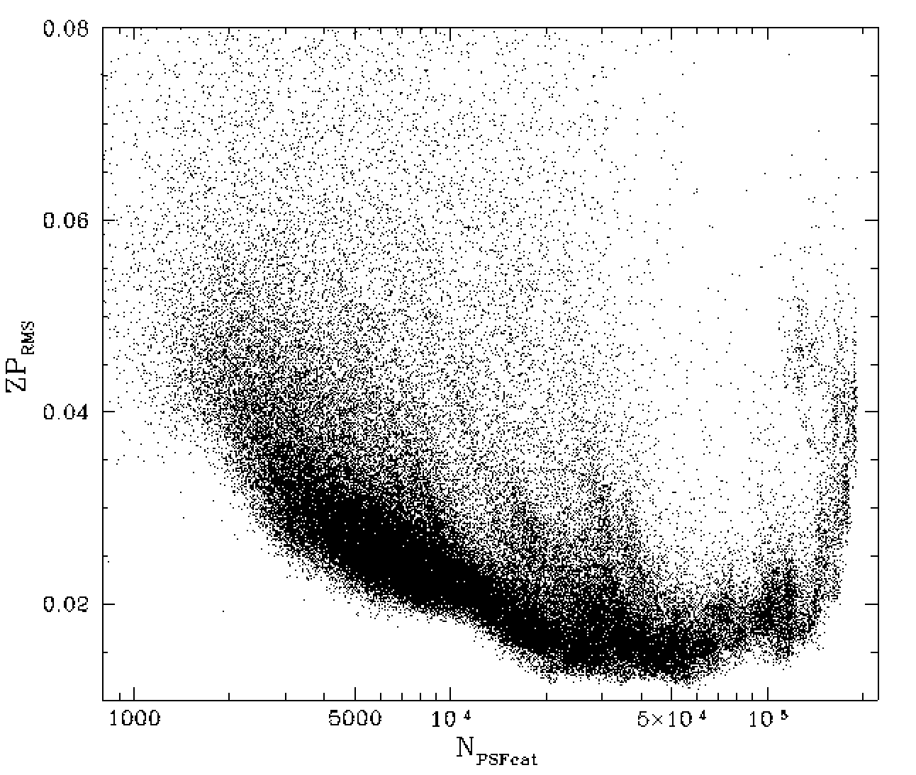
Zero point accuracy. A comparison between the number of PSF stars within a ZTF quadrant with the zero points RMS in that quadrant.
The number of calibrator stars is clearly related to the number of PSF catalog sources. In the plot above we show how the RMS varies with stellar density. Clearly when there are fewer than 1000 catalog sources we always have a ZP rms greater than 0.02. This is likewise the case in densely crowded fields with > 150000 PSF stars. Clearly if the zero points are not accurate at this level, the photometry cannot be. In fact, the photometry only reaches 1.5% RMS in fields with between 20,000 and 70,000 stars. Thus, in order to reach 1% or better, we have no choice but to improve the accuracy of the zero points using additional information.
Additional sources that limit the calibration accuracy include the degeneracy of PS1 colours for sources with g - r > 1.1 colours in the ZTF r-band calibration. As well as the very strong dependency of colour coefficients on reddening.
In g-band, the calibration is limited by large systematic variations between readout channels, as well as a software-based bias in the derived colour coefficients with skylevel and the number of calibrator stars (as noted above).
Strong colour and spatial dependency in PSF
As an intial test, a recent set of r-band data was selected under the assumption
that such data has better characteristics than older data due to improvments in
readout methods, linearity corrections, etc.
The first set of data was taken from 2020-04-29.
Tests were made to determine the approximate dependency of the zeropoints on
source airmass, magnitude, E(B-V), (r-i)_PS1. Results of the initials fits
provided photometry that was more poorly calibrated than current photometry.
Since the raw ZTF photometry is well known to included a magnitude
bias
when compared to PS1, an additional magnitude squared term was added to
account for this. This source is believed to be due to a combination
of non-linearity and the brighter-fatter effect.
This additional slight non-linear dependence is evident within the photometry
when we make a HESS diagram of the magnitude distribution.
However, even with the second order term the results of fitting r-band data
for a single quadrant (RC0) from an entire night is less accurate as the
current single image calibration.
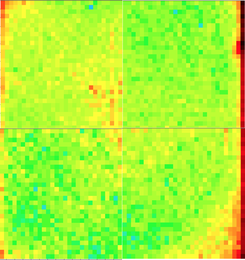
Nevertheless, when we spatially bin the residual differences between ZTF
and PS1 magnitudes we see the same structure as we had found
before.
This suggests that the spatial structure can now be determined on a nightly basis.
Although, this structure is clearly similar to the prior determination.
To determine why the newly calibrated photometry was inferior to the
current analysis we compared the distribution of photometry
in terms of magnitude, airmass, E(B-V), colour and time.
In the above plot we see that the ZTF photometry calibrated with on zero point
offsets is not symetric above the average zero point suggesting a bias with source
brightness. The photometry including the calibrated colour coefficients is nearly
symetric. However, in the middle plot we some significant outliers below the
average zero point that are not seen in our new calibration since the new
calibration includes reddening.
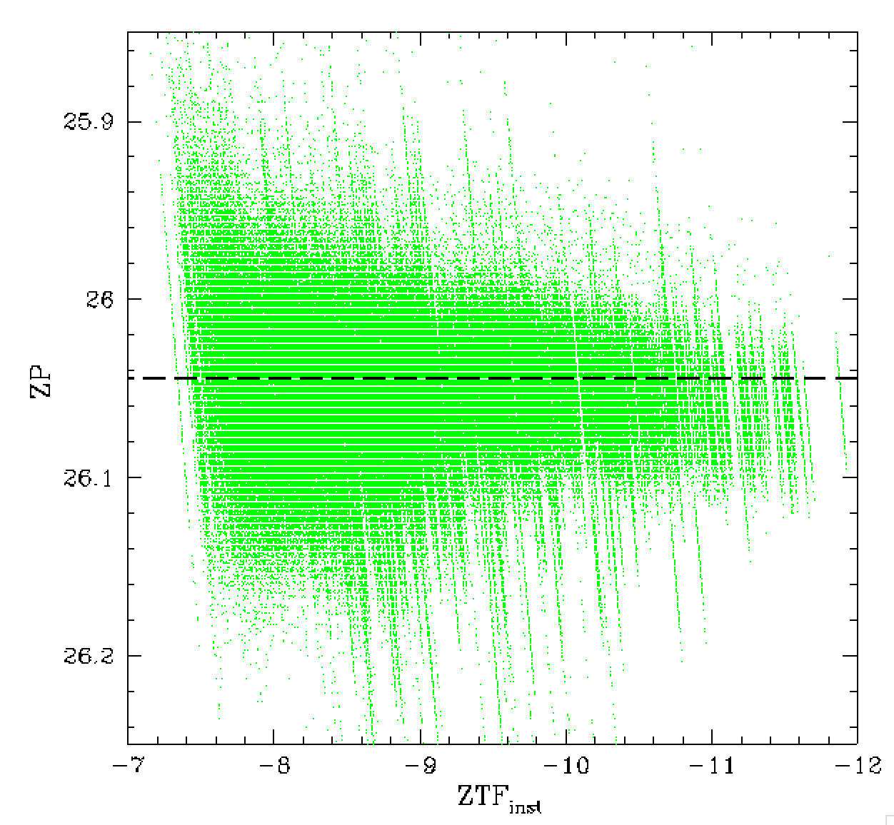
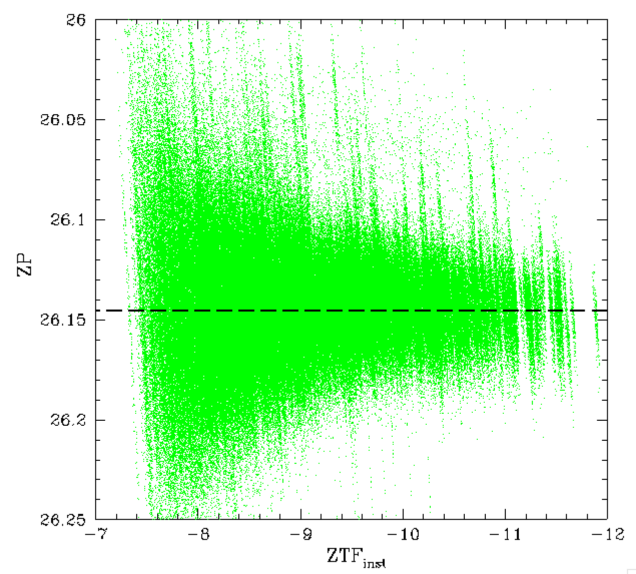
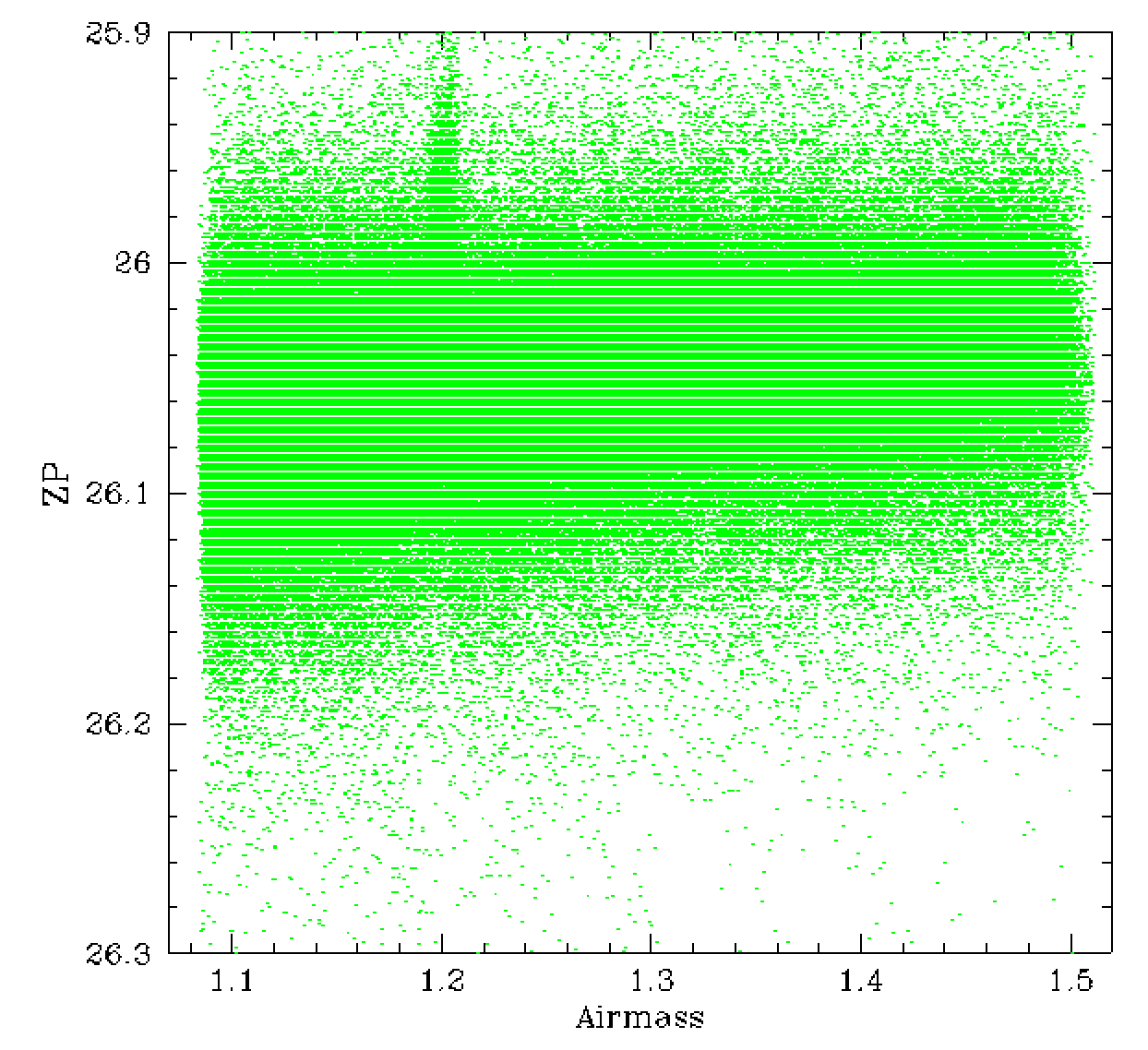
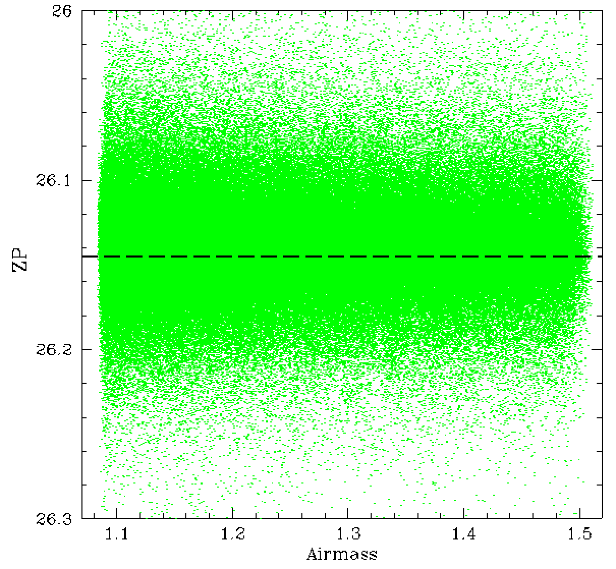
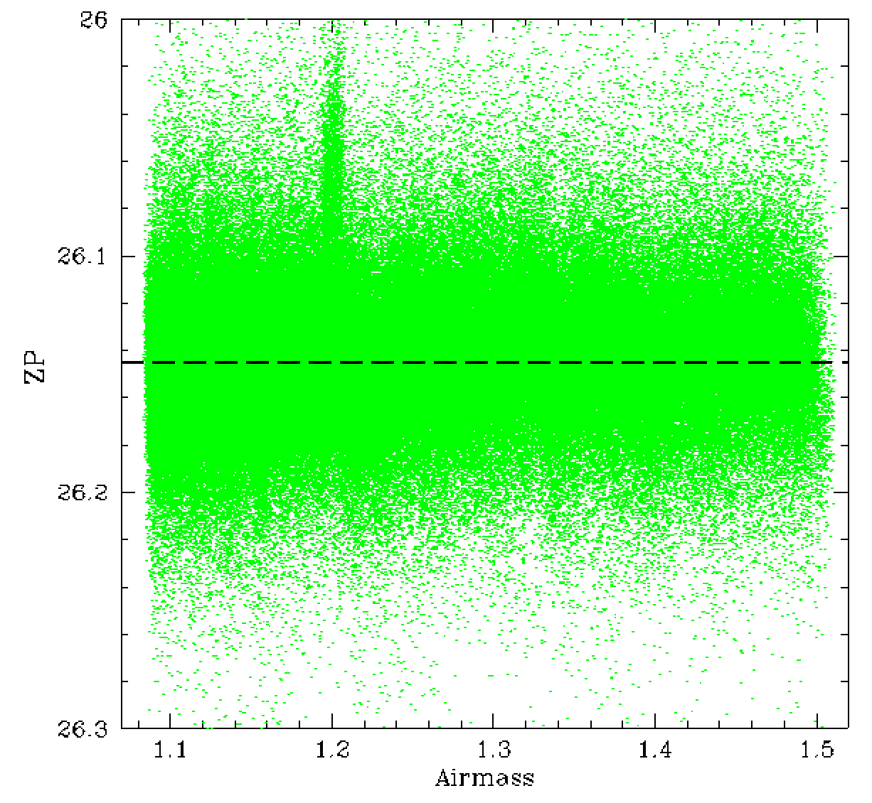
In the plot above we see the colour dependence of ZP calibrated data with
increasing airmass. That is, the zero points decrease due to
extinction as expected. This effect is corrected in the current ZTF
calibration include colour coefficients.
The new Zuber calibration removes the trend, but exhibits more
structure than the current calibration. In particular, some
significant outlying data is seen.
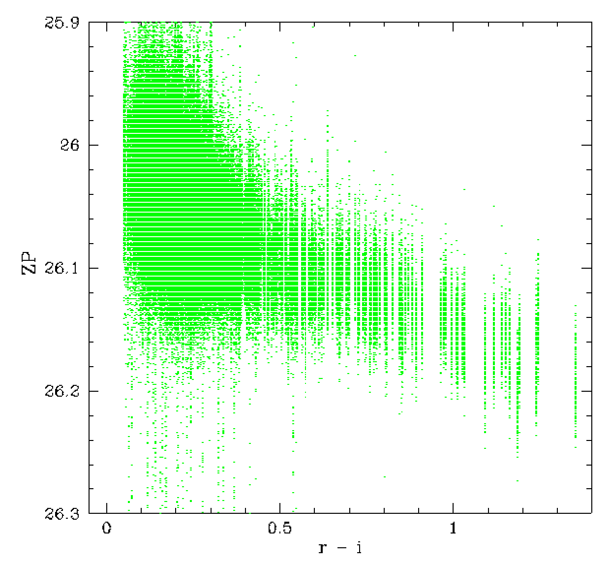
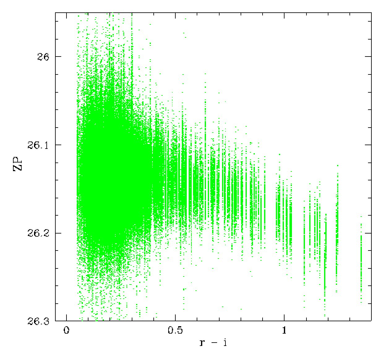
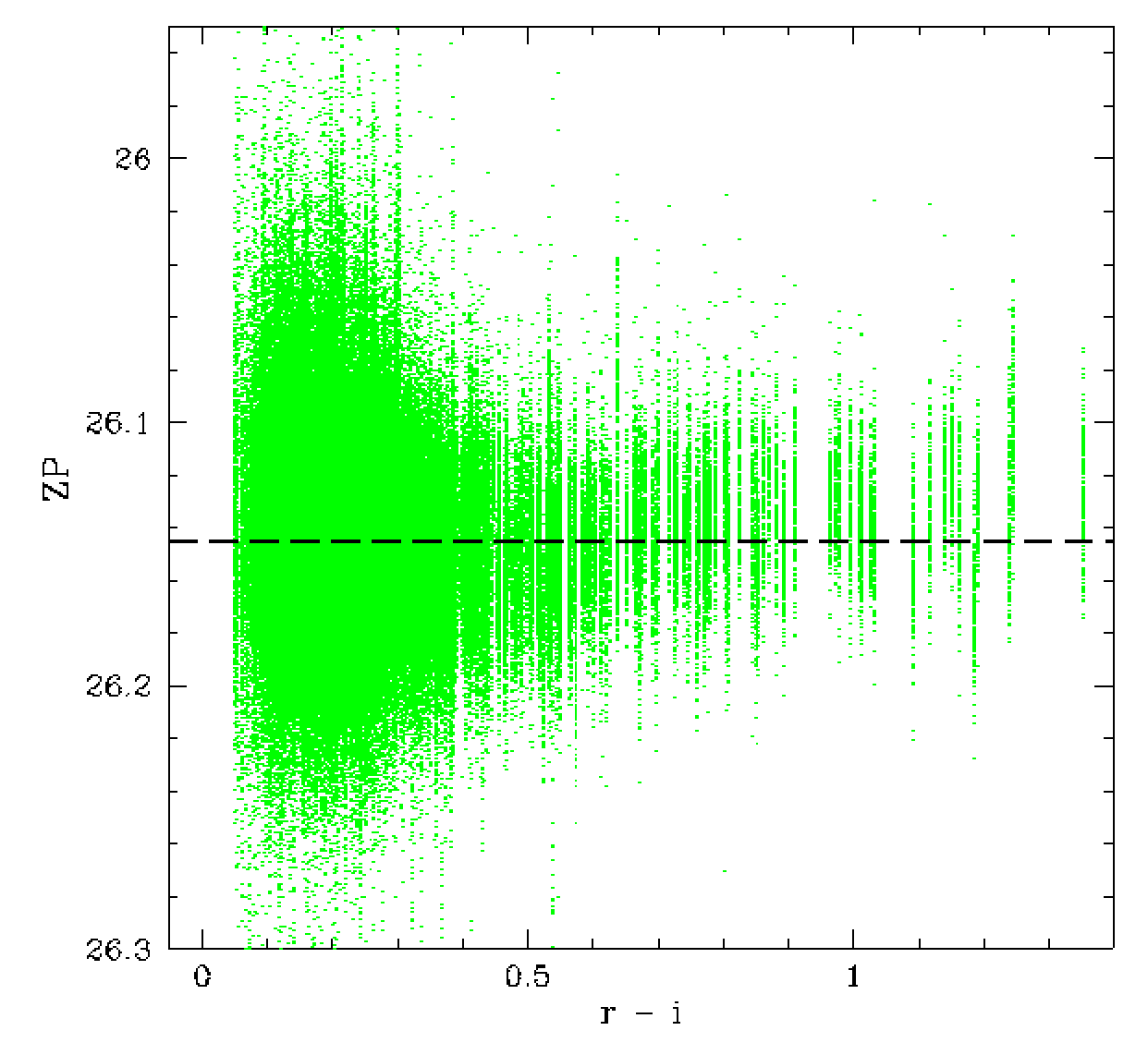
In the plot above we see how the data without colour calibration exhibits
a very strong trend with colour since ZTF filters do not match PS1 filters.
In the middle plot we see that even the current colour calibrated data still
exhibits a strong colour trend for the small number of calibrator sources with
r-i > 0.8. In the new calibration we see improvement. However, the calibration
is clearly still not ideal.
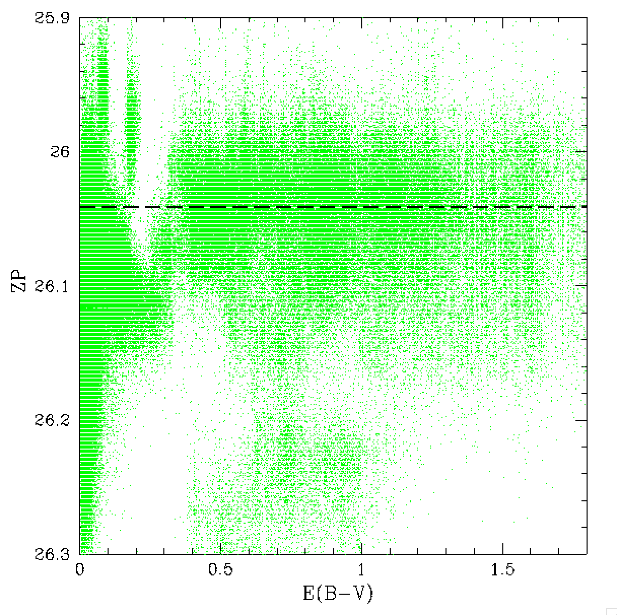
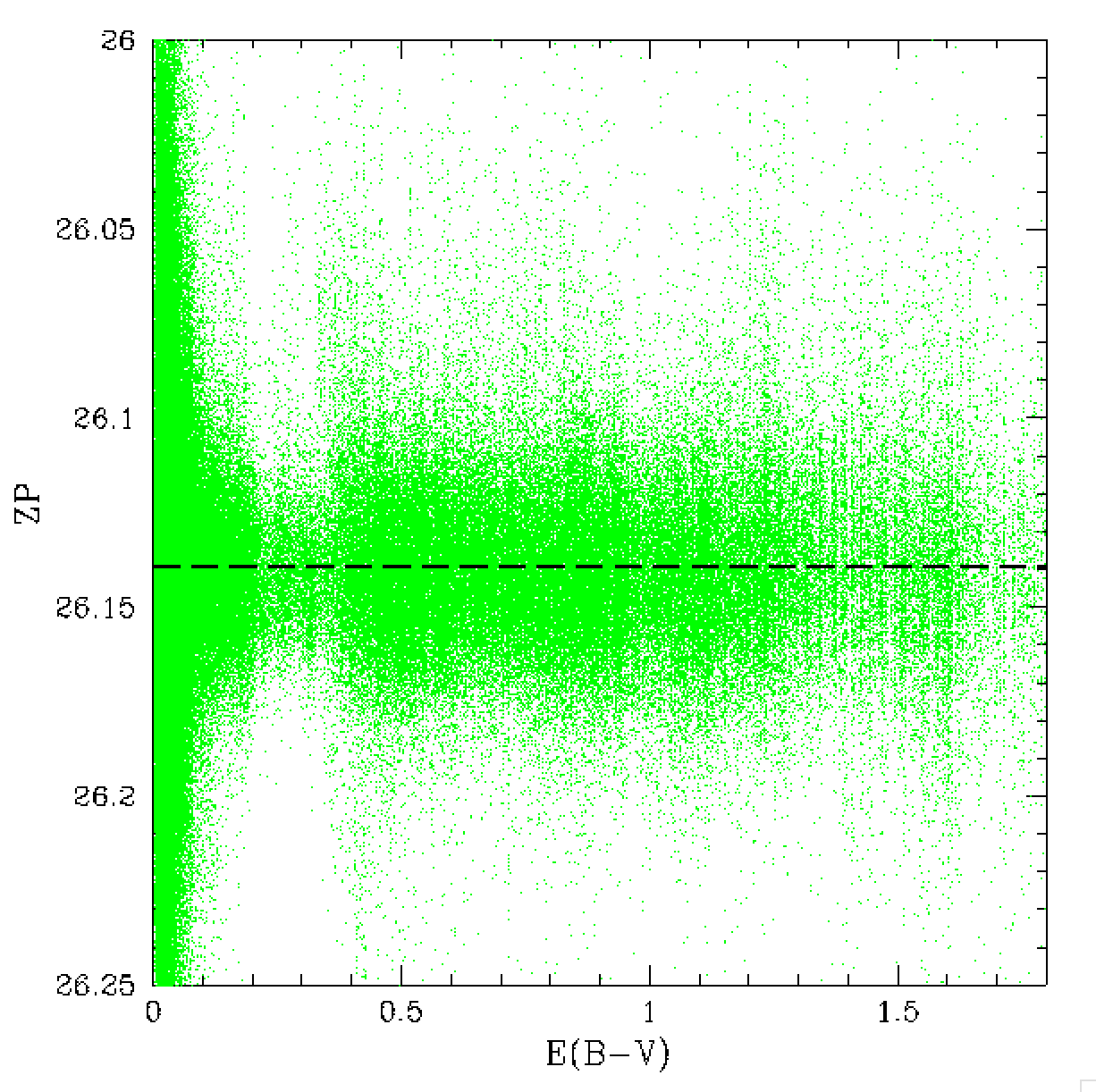
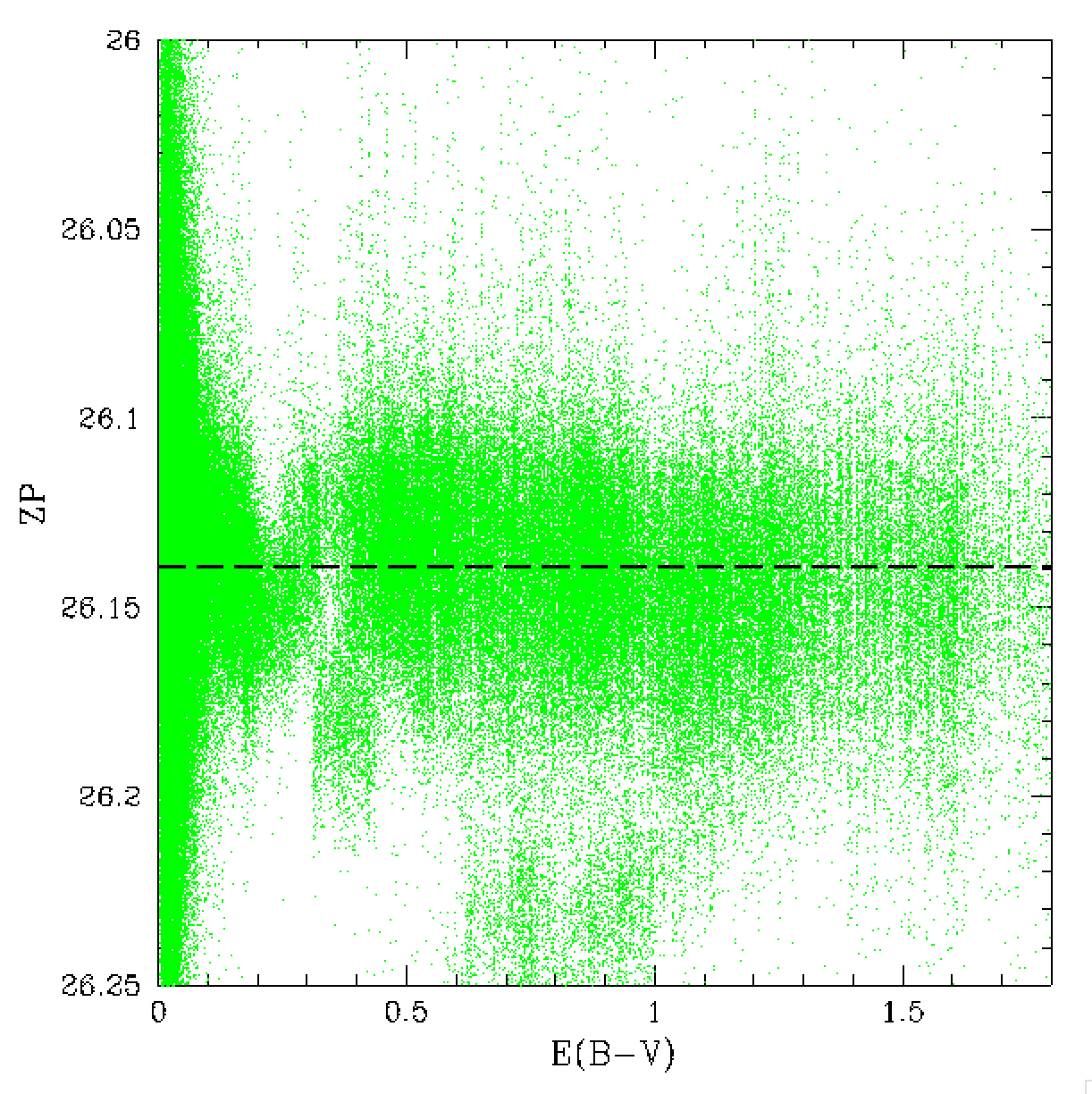
In the plots above we see significant structure in the calibration
versus reddening for both the current calibration without colour
correction and the new Zubercal. The main feature is a dog leg
in the values at around E(B-V)=0.15. This feature was seen g-r colours
in our prior work.
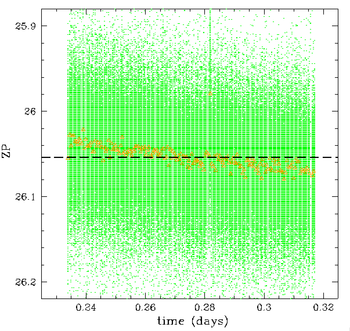
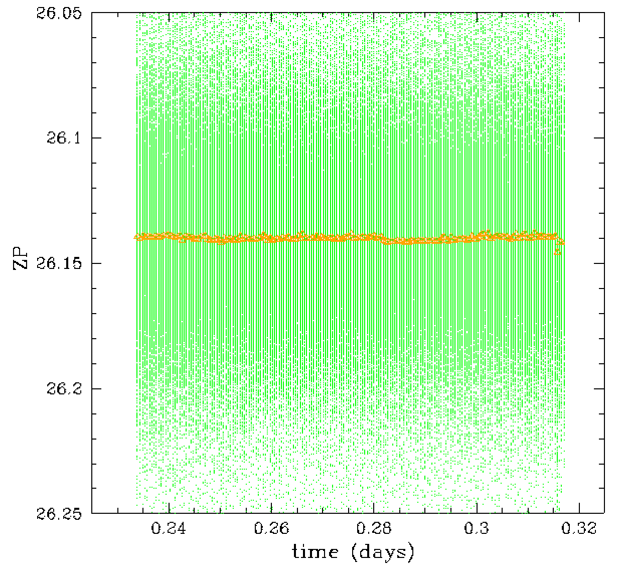
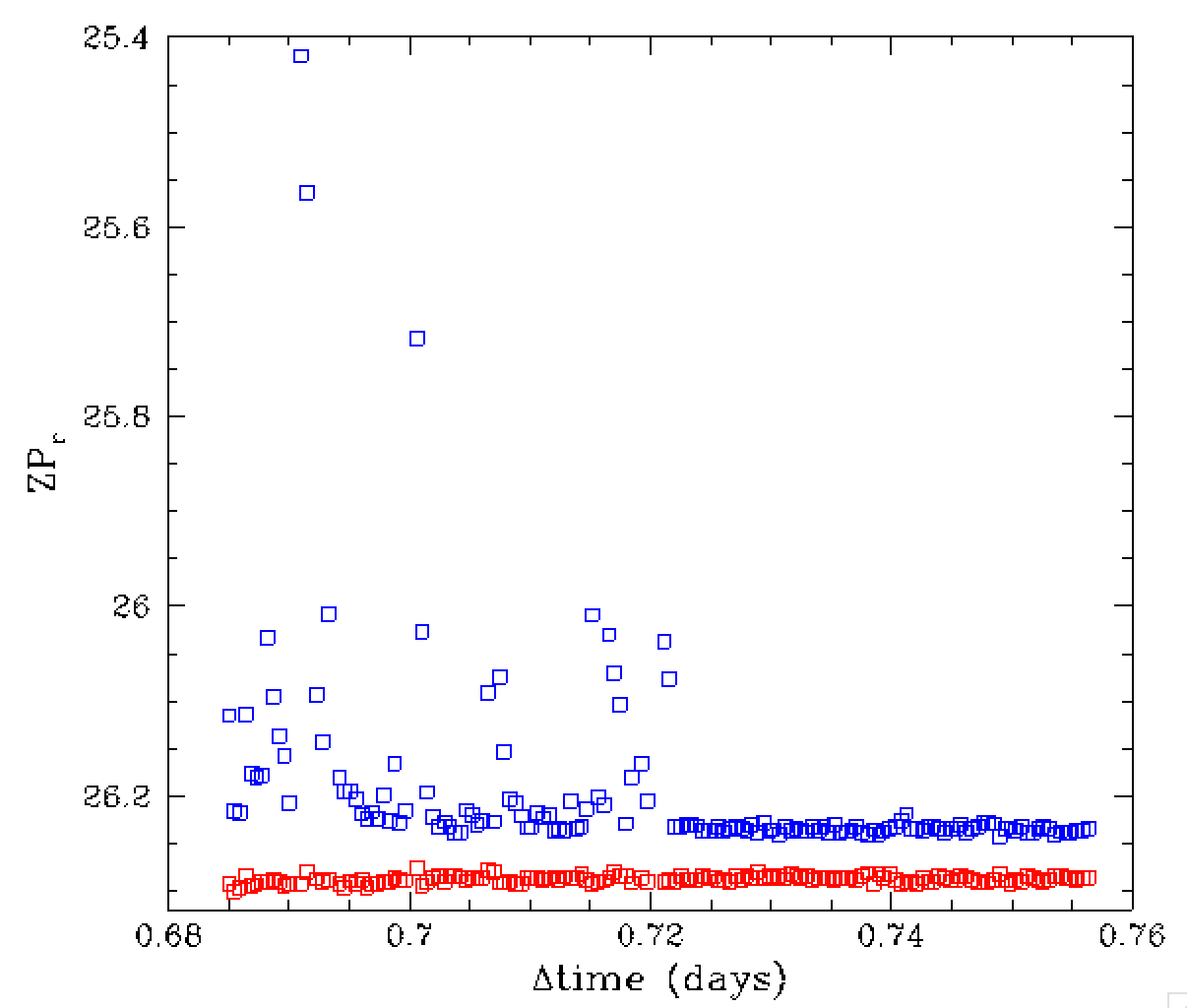
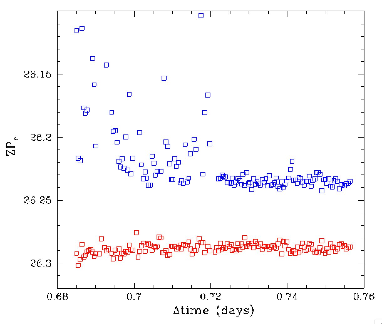
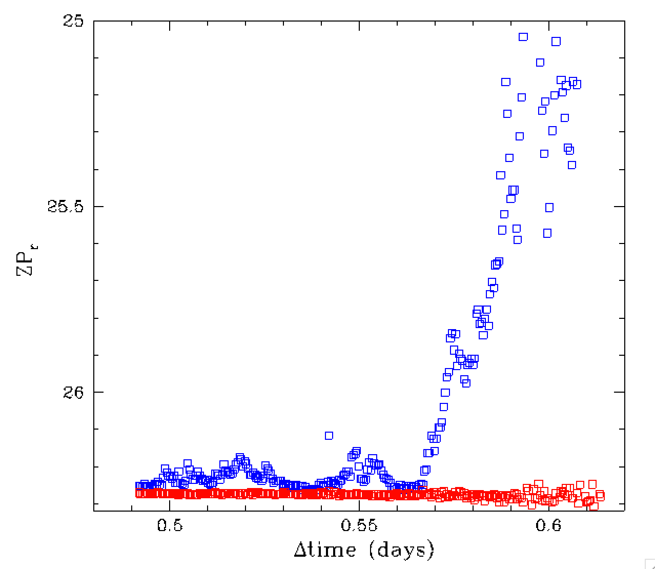
In the above plots we see how the zero points change with time.
The data without colour calibration shows a significant overall
trend, due to airmass, along with additional structure.
The photometry calibrated with the current systems shows very
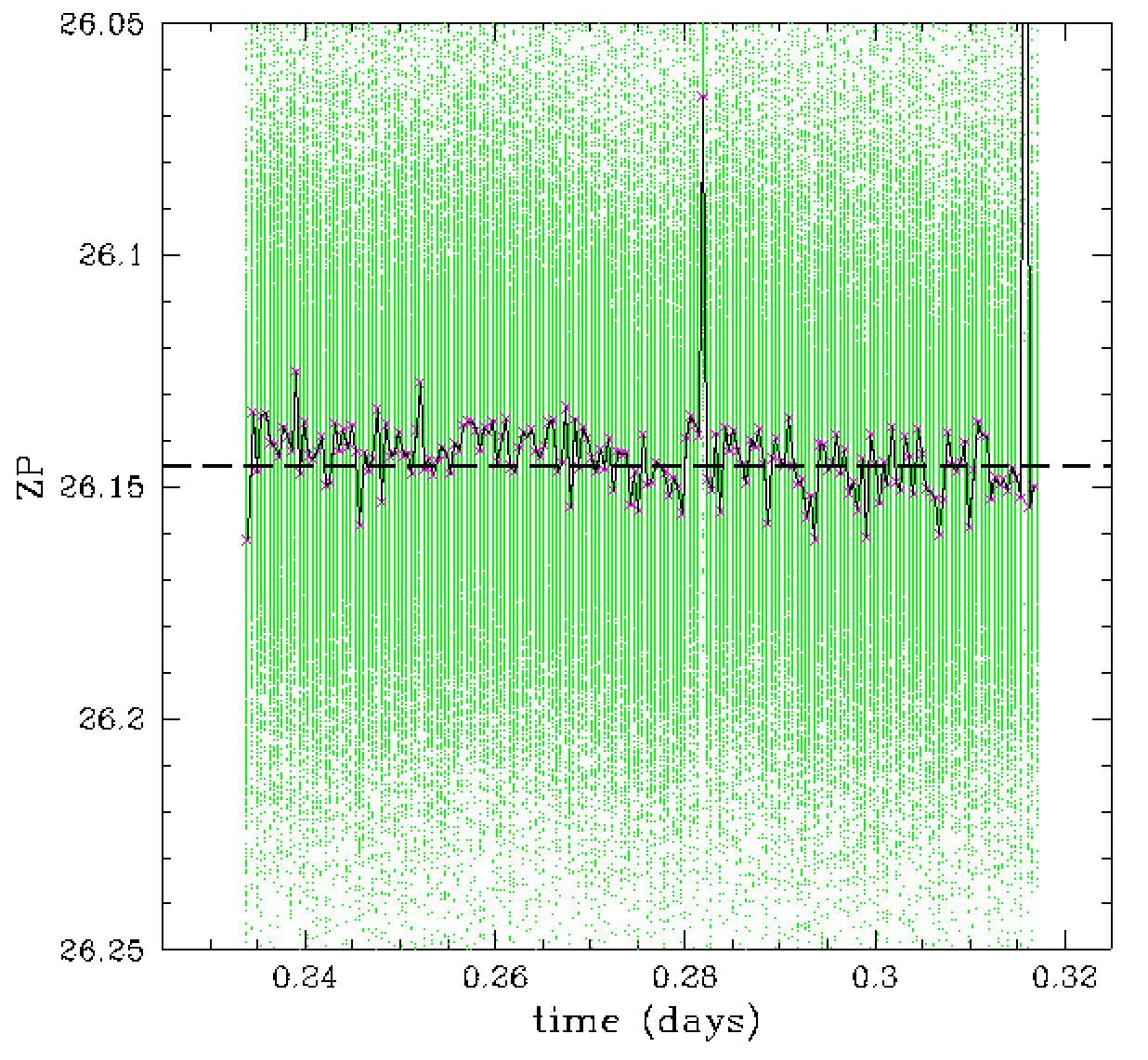
little variation in average zero points with time. The new
Zubercal calibration shows the same kind of rapidly varying
structure as the left plot. In the right plot we see two images
have low zero points that clearly stick out.
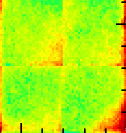
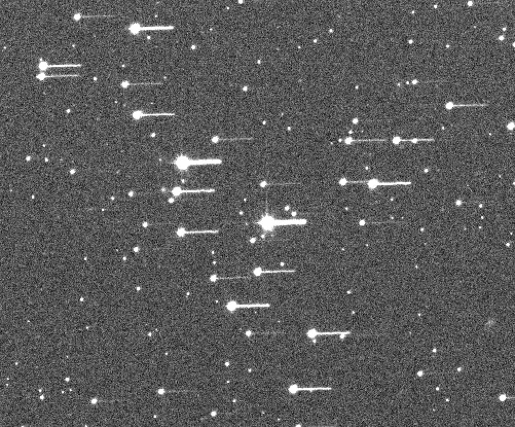
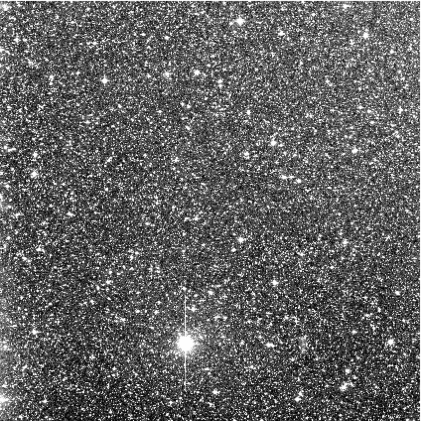
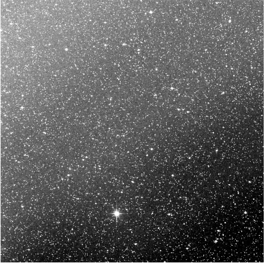
In the above images we see the reason that the two image stick out in terms of their
zero points. Notably these two bad qaulity images are not obvious in the distribution
of values with current calibration due to the calibration not requiring any consistency
between successive images.
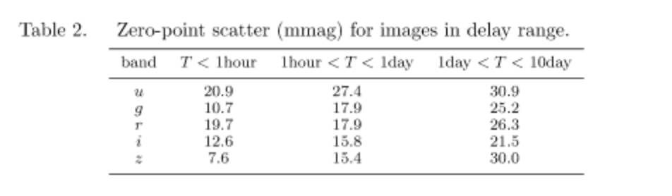
The most important point of the ZP vs time plots is that the
zero points vary significantly on short timescales. In the following
table (from Stubbs et al.?) we show the variations in zero points
that have been determined for a range of different timescales.
For the table we see that a 0.02 mag variation is not unexpected in
r-band observations on timescales of less than 1 hour. Thus, the
observed variations are expected, but not accounted for in our
initial Zubercal calibration.
Further evidence for very significant changes in ZP caused by clouds is seen
in our earlier
work.
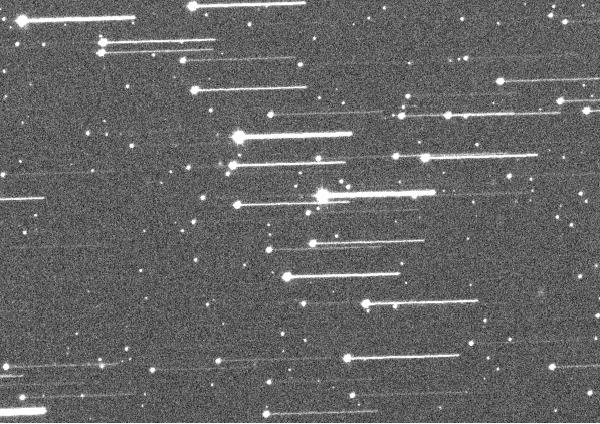
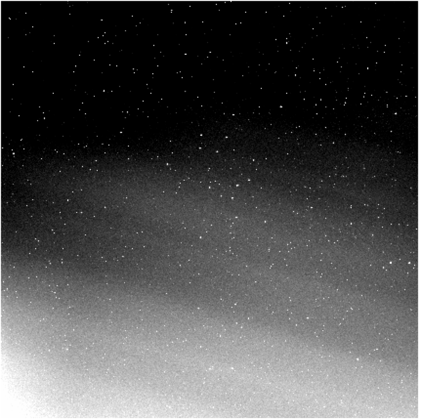
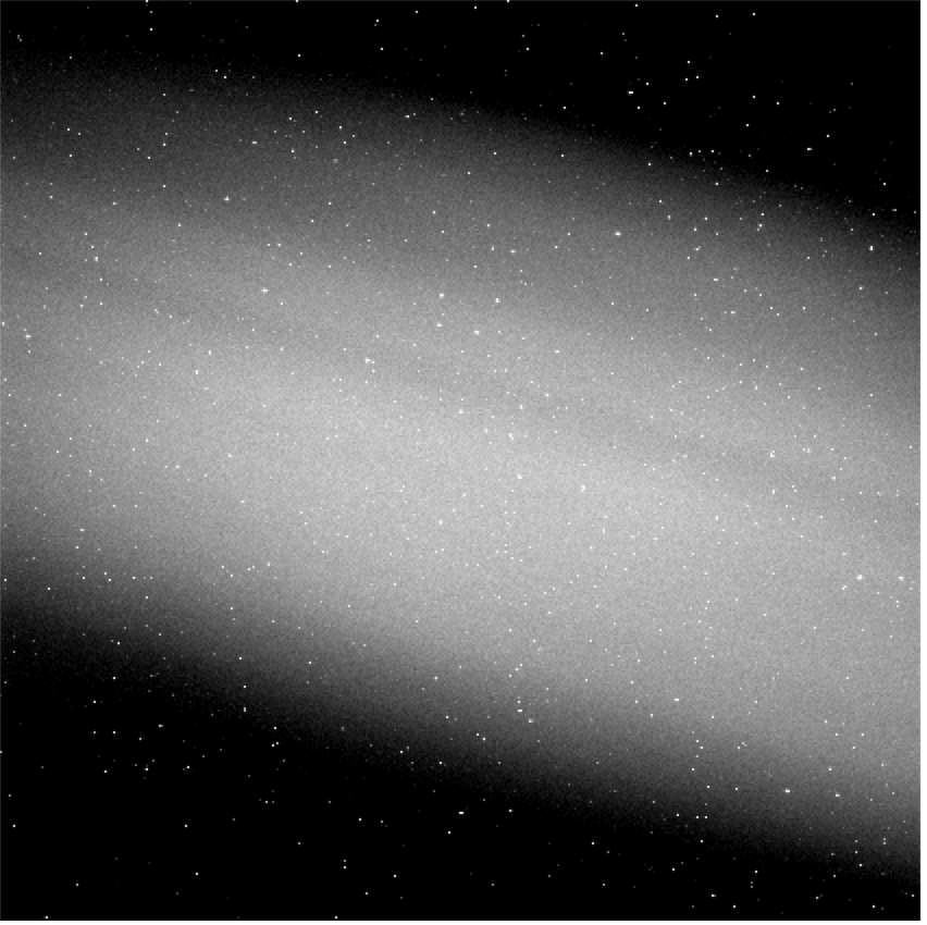
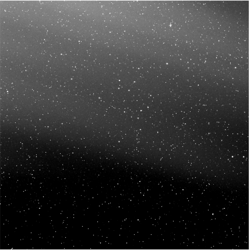
The spikes suggest that in ZTF data far greater variations in image depth
of over a magnitude are not uncommon. However, the presence of cloud are not
typically evident in the images since skylevel only show when the moonlight,
or other external sources, are present as shown below:
In order to test the importance of the transparency variation induced zero point changes
we determined the nightly average zero point and subtracted the difference between the
Zubercal frame average.
As we can see from the above plot, correcting the zero points to the frame
average produces an accuracy the same as the current calibration. However,
more importantly, even with all the noted changes it does not improve on it.
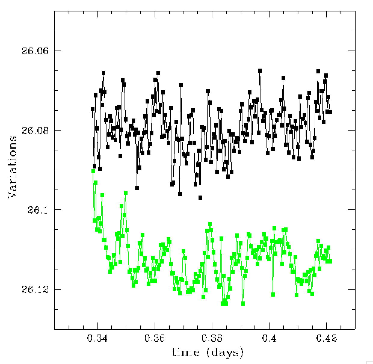
We found that the zero point variations were slightly correlated with the
focus. This is shown in the figure above where we plot the variation in
the photometric zero point over time along with a scaled variation in
focus over time. Thus variations in focus may be of slight use in
determining the variations in the zero point.
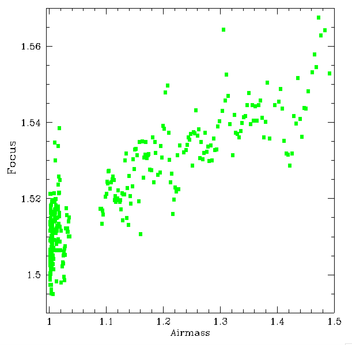
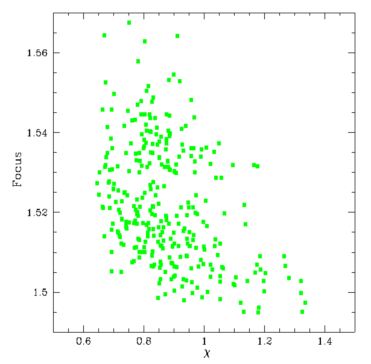
In the above plot we see that there is a strong relationship between
the focus and airmass and a moderate relationship between focus and
the averaged photometric Chi values for a frame. The first plot most likely
just tells us that the focus is varying with time as the airmass does,
while the second plot tells us that the PSF model we used was not ideal
for the observations that were taken at lower airmass (noting values
given in the left plot).
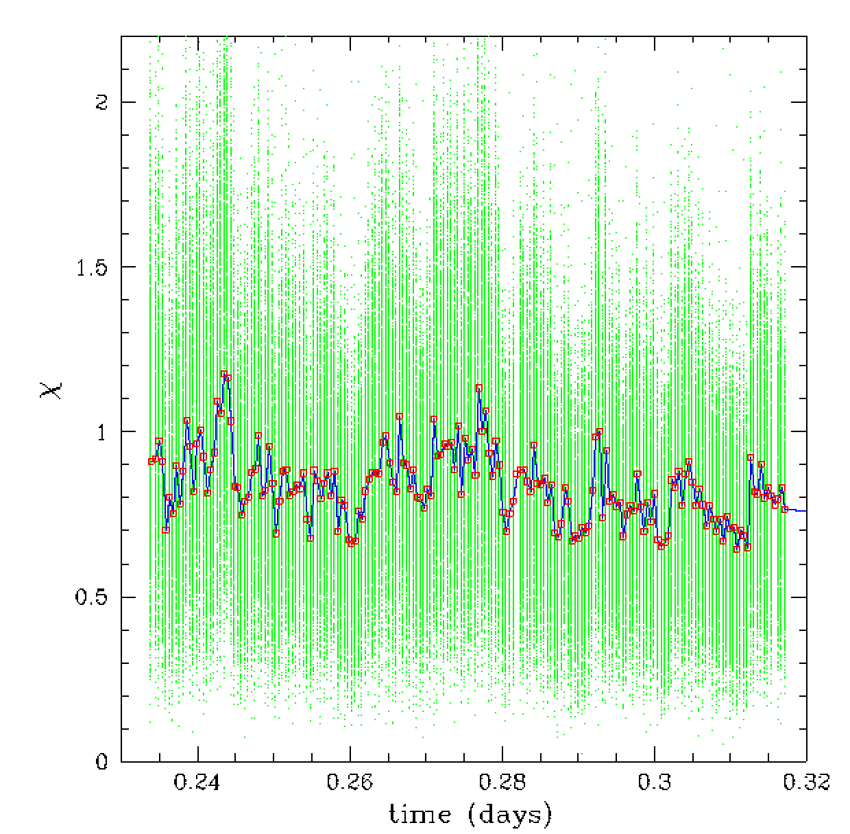
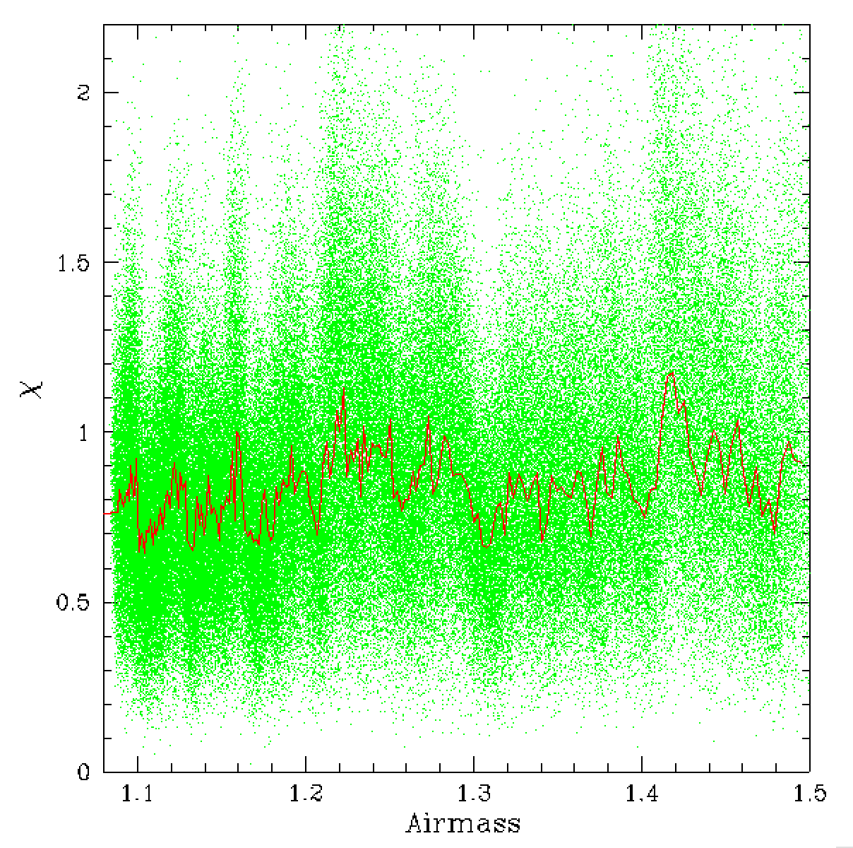
In the plots above we see the strong variation in the distribution of
Chi values for repeated observations of bright calibrators (and the
average) in field 614, over time, and also versus airmass. The Chi variation
with airmass simply reflect the decrease in airmass for these particular
observations with time.
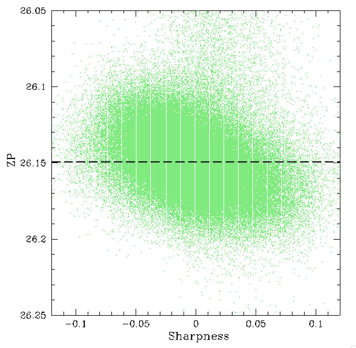
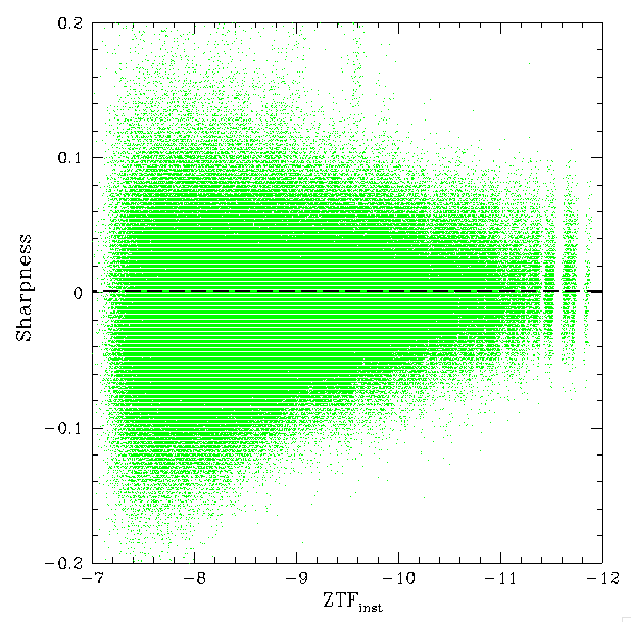
In the figures above we show the importance of the PSF sharpness
parameter. We see that these bright sources exhibit a strong trend
in sharpness that affects the measured magnitudes.
In the right plot we see that the distribution of sharpness changes
slightly with magnitude. These results follow the results of our
prior analysis. However, here we did not find significant variation in
chi and sharpness with colour. This is likely due to the limited
nature of this data set.
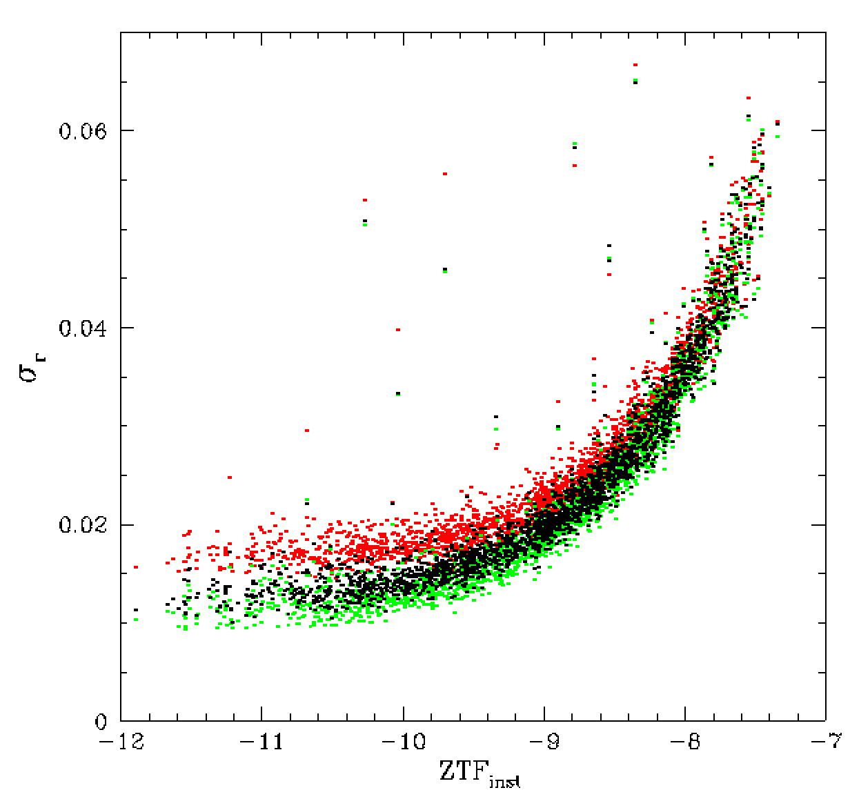
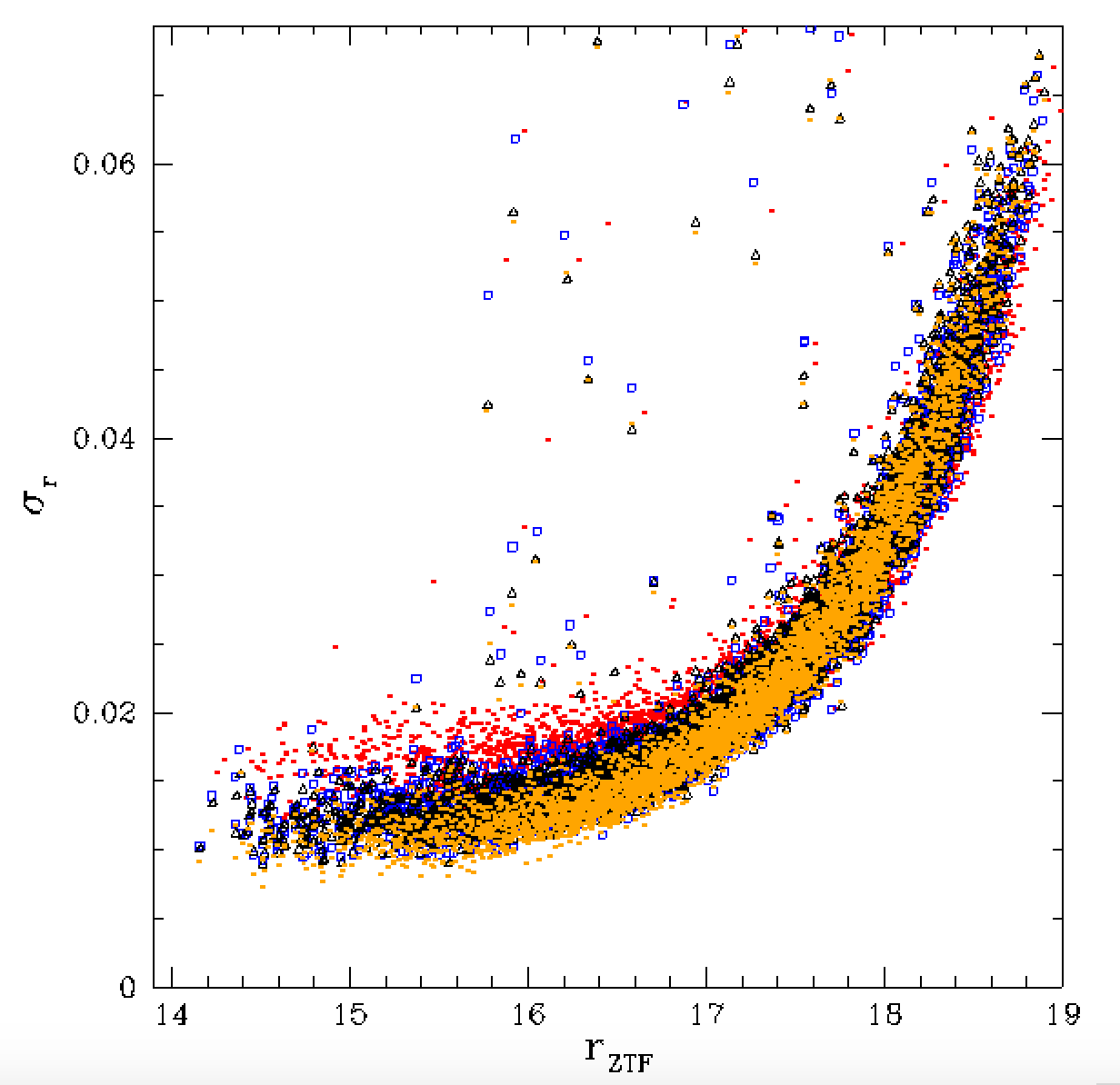
When we add chi and sharpness measurements to our fits we see improvement
in our calibrations. In the above plots we see that we are finally reach a
1% calibration level for bright stars observed in an uninterupted sequence.
In fact, even the Zubercal without fitting chi and sharpness terms show
less scatter than the current ZTF calibration.
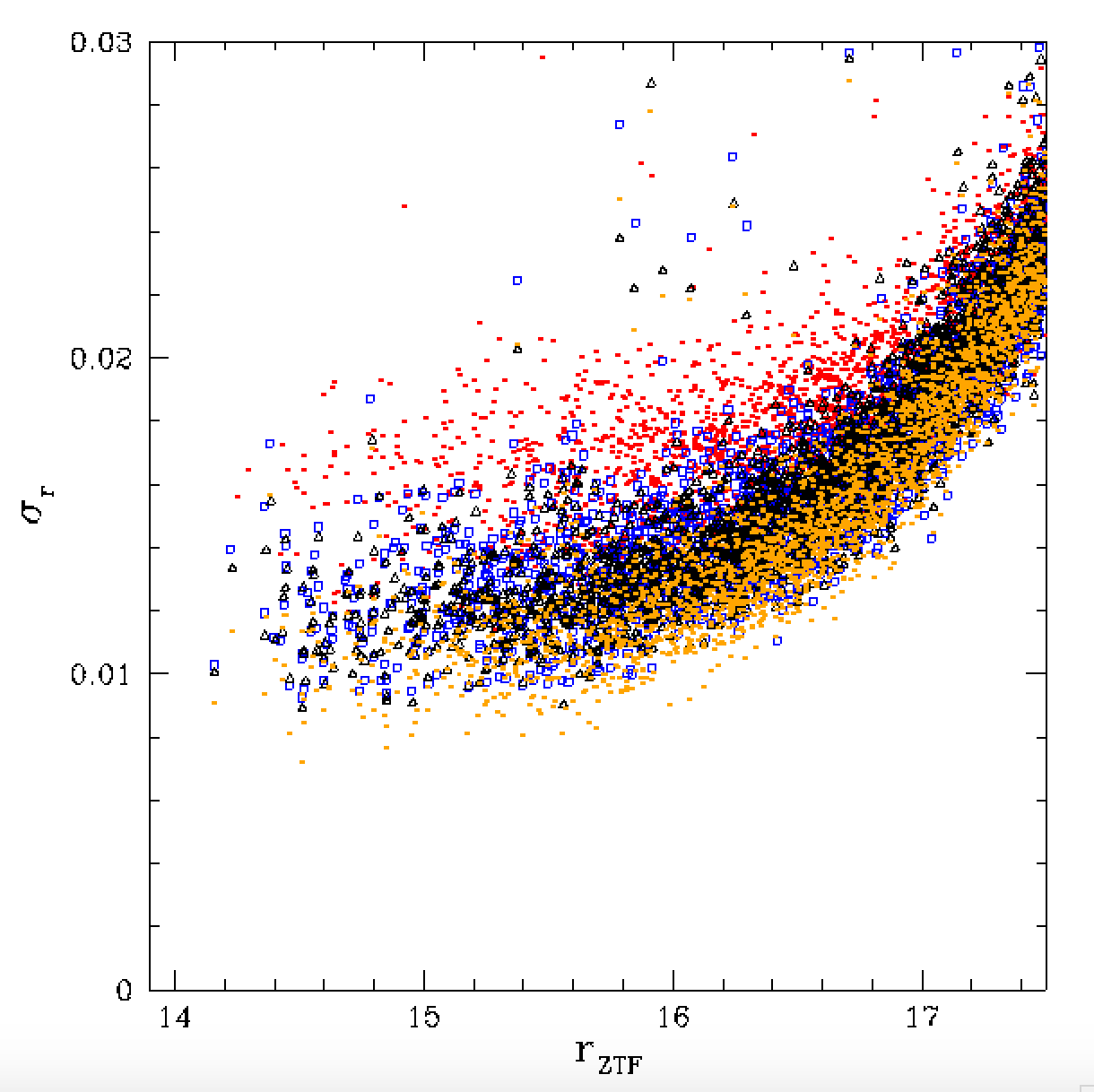
Notably, at the faint magnitude end, the calibrations do not improve
the scatter. Indeed they all appear slightly worse. Even the current
calibrations. Given that this photometry is dominated by statistics
it is unclear how much improvement in scatter can be made with any
calibration. It is also worth noting that there are numbers of
calibrator stars above the main locus. These may be variable stars
or edge stars.
The calibration improvements with the addition of chi and sharpness parameters
are not so clear in the fields that were not measured in sequence since those
fields were significant affected by transparency changes as noted below.
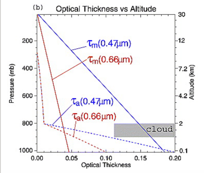
In the plot above we show the various atmospheric components responsible
for transparency variations.
Considering this we can see that there are numerous possibilties for
atmospheric changes to significantly impact photometric calibration.
In addition to these components, clouds create a grey (wavelength
independent) extinction that can be complete in optical bands.
Considering the locations of the various atmospheric components we note that
most aerosols are trapped in the boundary layer, approximately 2 km thick
while Rayleigh scattering occurs over full atmospheric scale height.
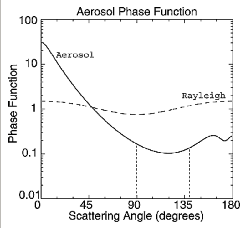
These two components also have very different scattering phase functions
as shown above. That is, light interacting with aerosols is forward scattered
while Rayleigh scattering is much more isotropic.
The amount of scattering is dependent on speciation. For example,
there is approximately a factor of three varation in Rayleigh cross
sections from H20, O2, N2, to CO2. This suggests that factionally varying
atmospheric water content may vary the amount of Rayleigh scattering
at a given pressure (or airmass). However, this variation has been found
to be 0.2% at 500nm.
We further note that atmospheric component changes, such in Rayleigh scattering
due to pressure changes and O2 variations, have been found to stable over
moderate timescales, while seasonal varations in O3 has an even smaller
effect.
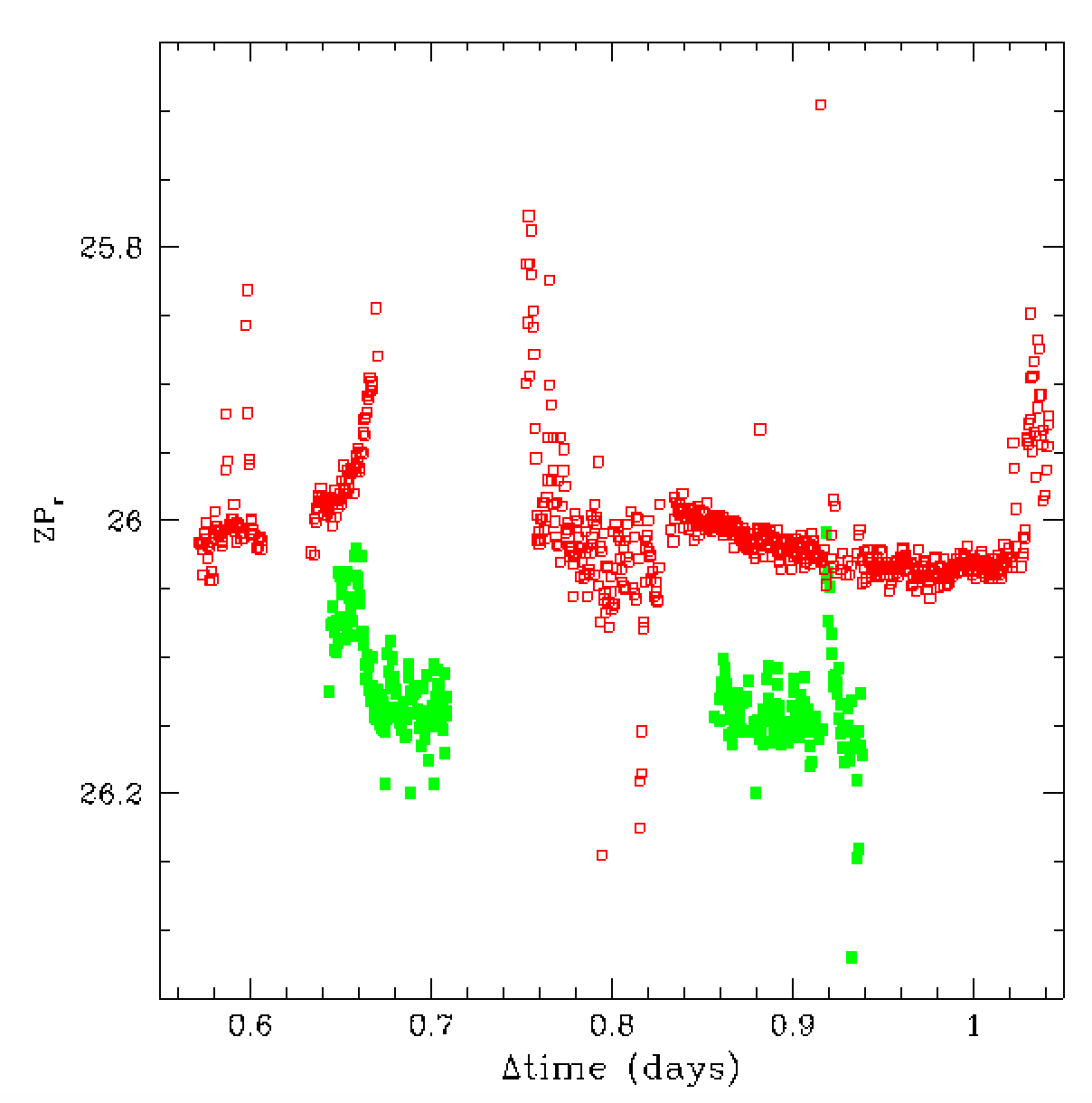
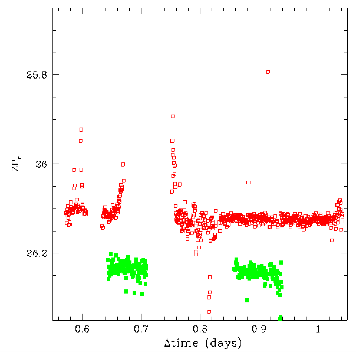
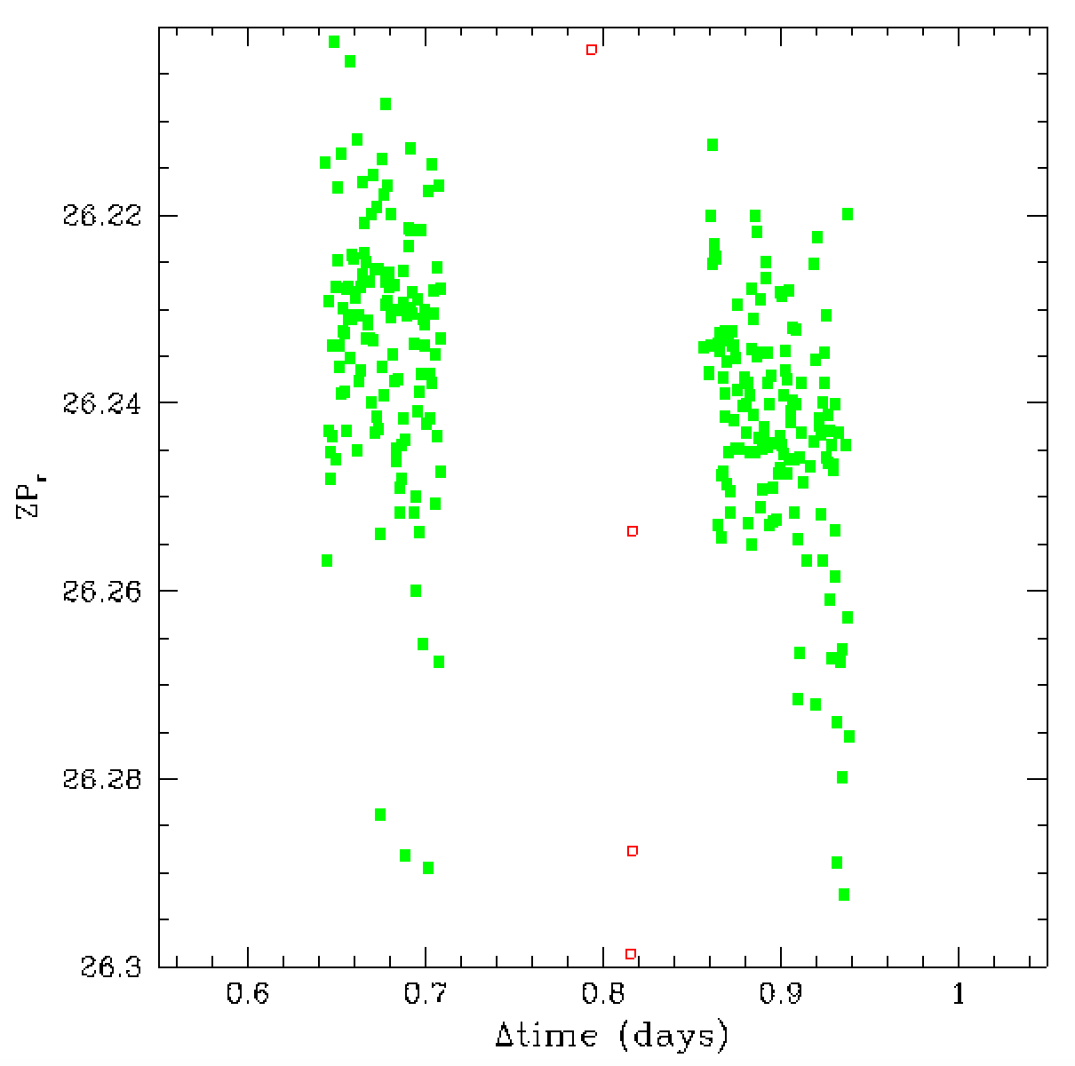
In the figures above we compare how the zero points vary overtime.
The left figure shows significant variation since airmass and
reddening are included in the zero point. Removing these terms
from the ero points in the right plots we less variation
in some parts of the plot. However, we see that there is
still significant variation.
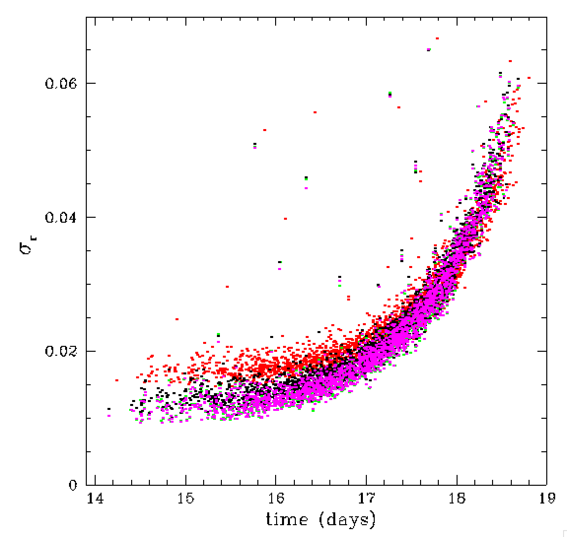
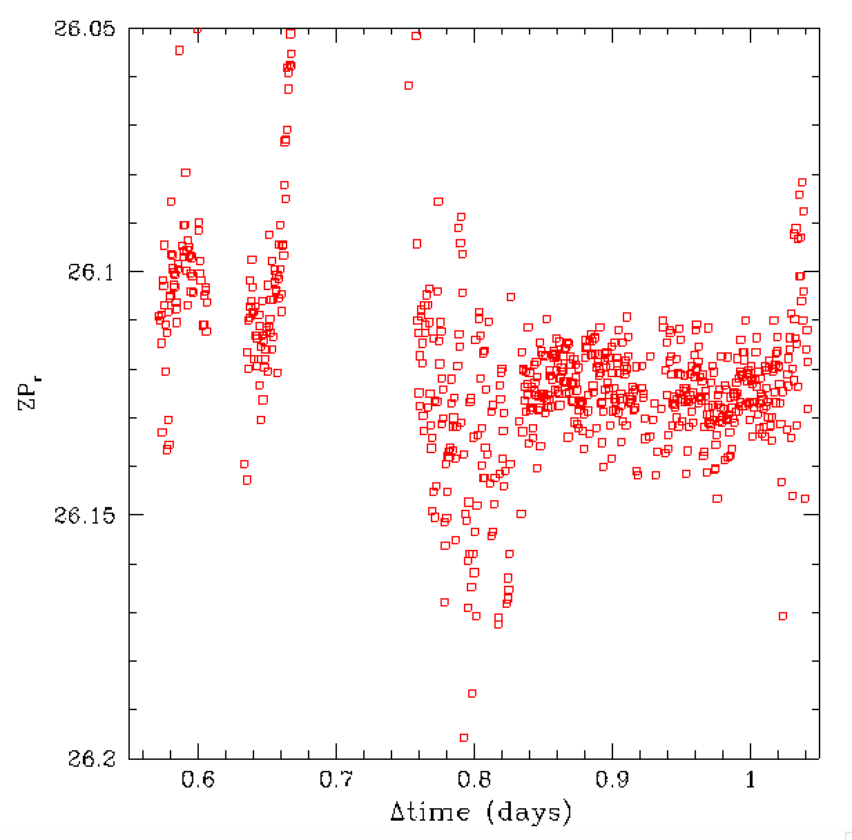
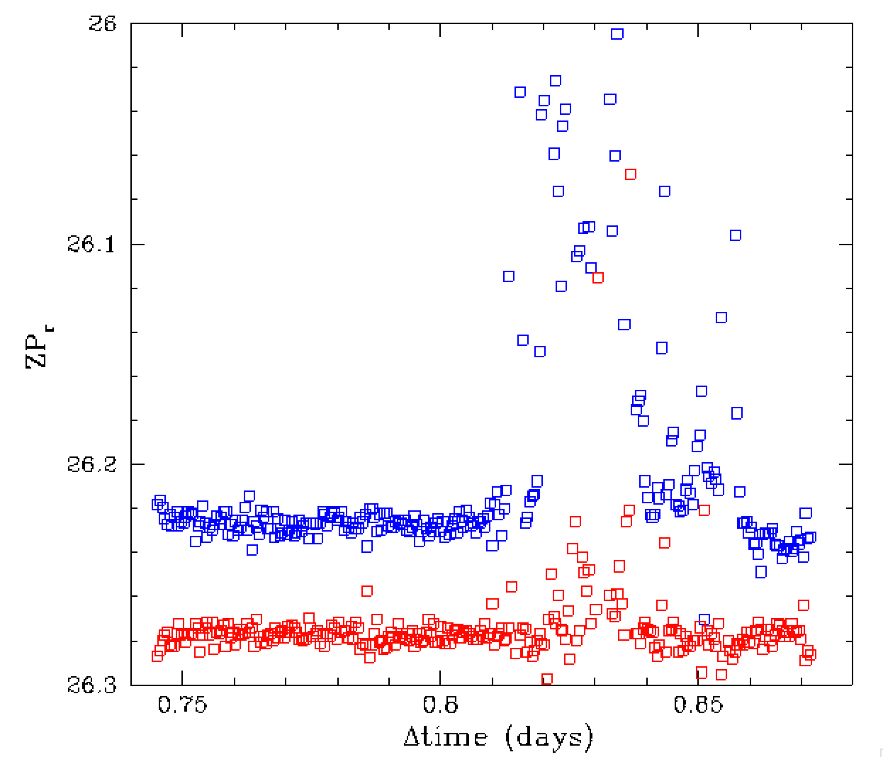
When we zoom in or the zero points we see that there is still significant
variation. This variation is significant even when observing the same
field repeated as seen in the red points between 0.85 and 1 day.
When observations were taken different fields at different locations
0.75 < t < 0.85 the variation are larger. However, the variations
in the green points in the left plot are also different fields.
These variations, such as the rise near t = 0.65 days, are actually
caused by transpancy changes due to variation in clouds, water and
aerosols.
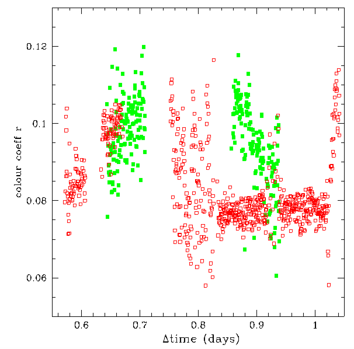
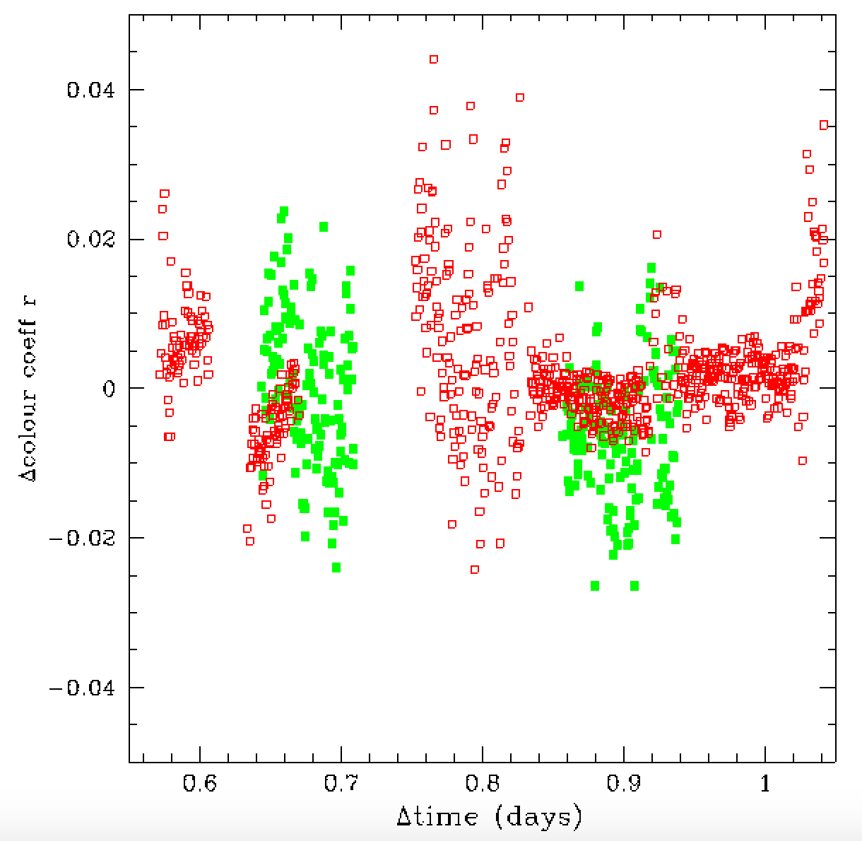
In the plot above we show the colour coefficents determined during the
regular calibration as well as those corrected for the airmass colour
term and reddening. Here we see that the colour term is changing
over time. This suggests that the cause of the transpancy variation
is not clouds (which produce grey extinction). This also tell us
that the extinction on this night cannot be fit with a single colour
term. Furthermore, the photometric variations do not obey a simple
linear model where atmospheric extinction is linearly varying with time
(as assumed by in Ubercal calibrations of SDSS and PS1).
Thus, to account for this a much more complex time dependent model
is required in the presence of vary transperancy (i.e. non-photometric
data).
For each image sequence we determined the average and RMS
scatter in the airmass-corrected ZPs, colour coefficients,
sky levels, FWHM, ellipicity and position angle. Initial checks
of this data showed that there was a very broad range on behaviour
during these image sequences.
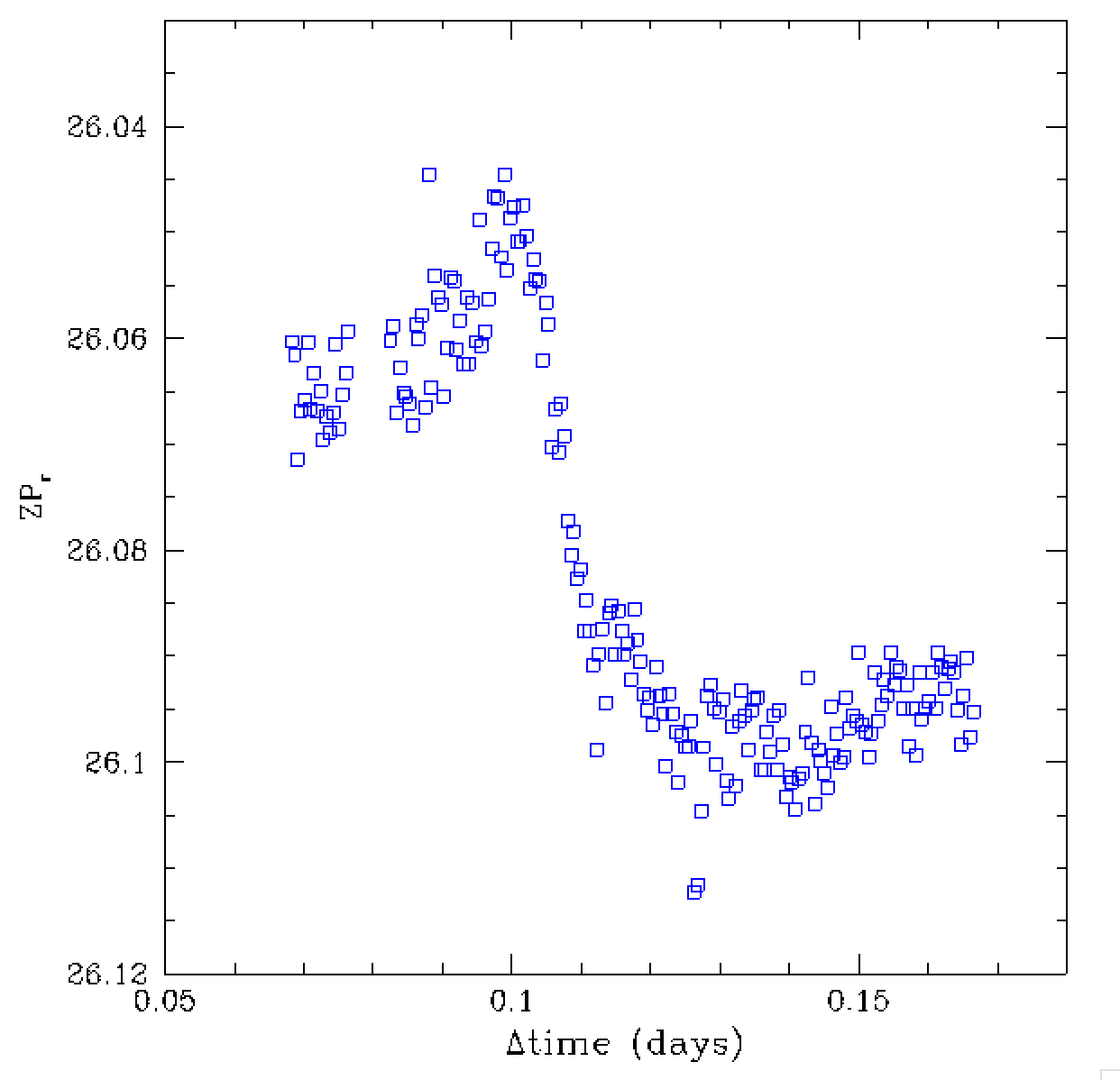
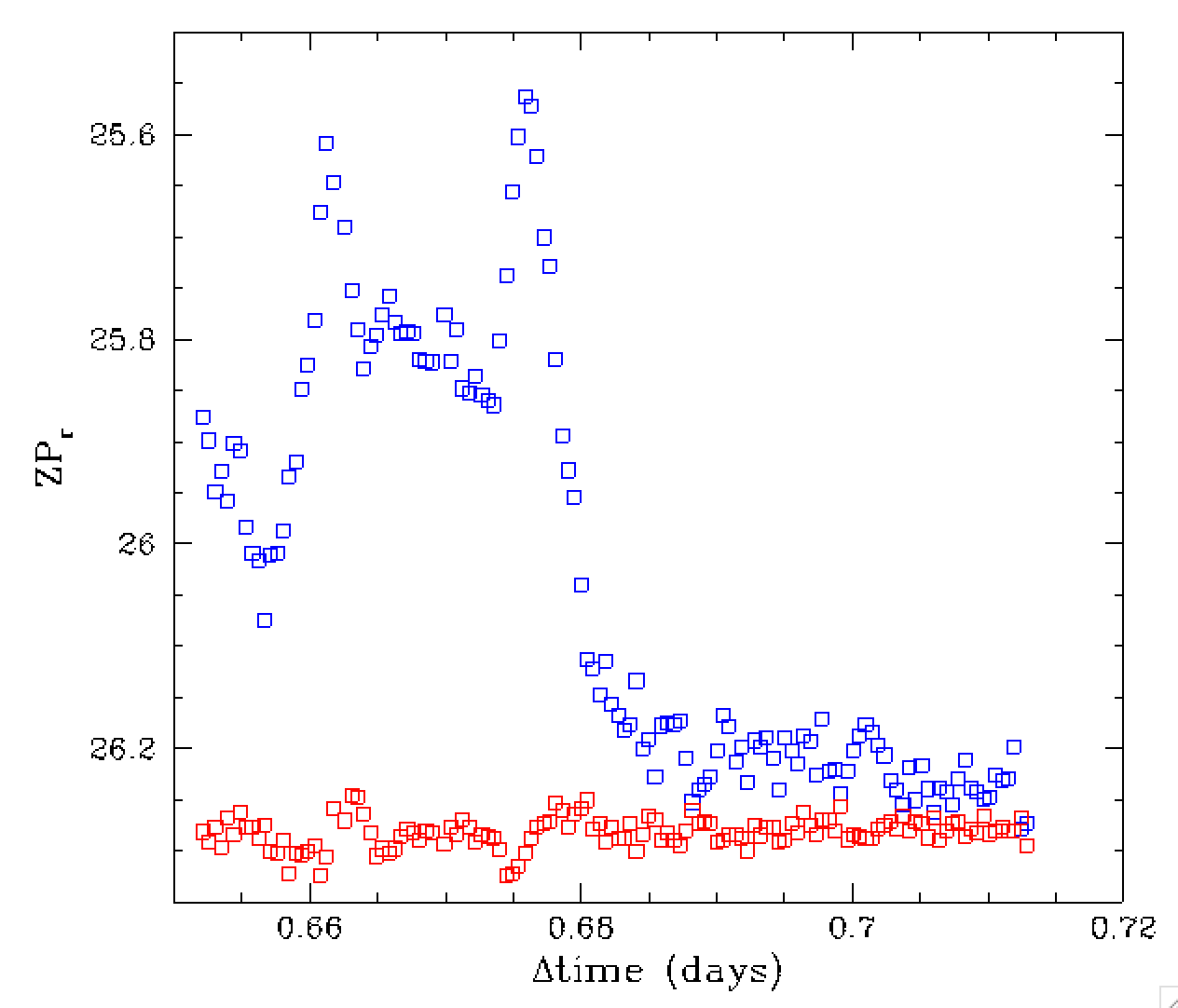
In the plots above we see an example of set of continous observations for
a single field (and quadrant). Over this time we see that atmospheric variations
give rise to a complex structure of image ZPs that clearly cannot be
approximated as a linear or even quadratic variaton over time. Note, the
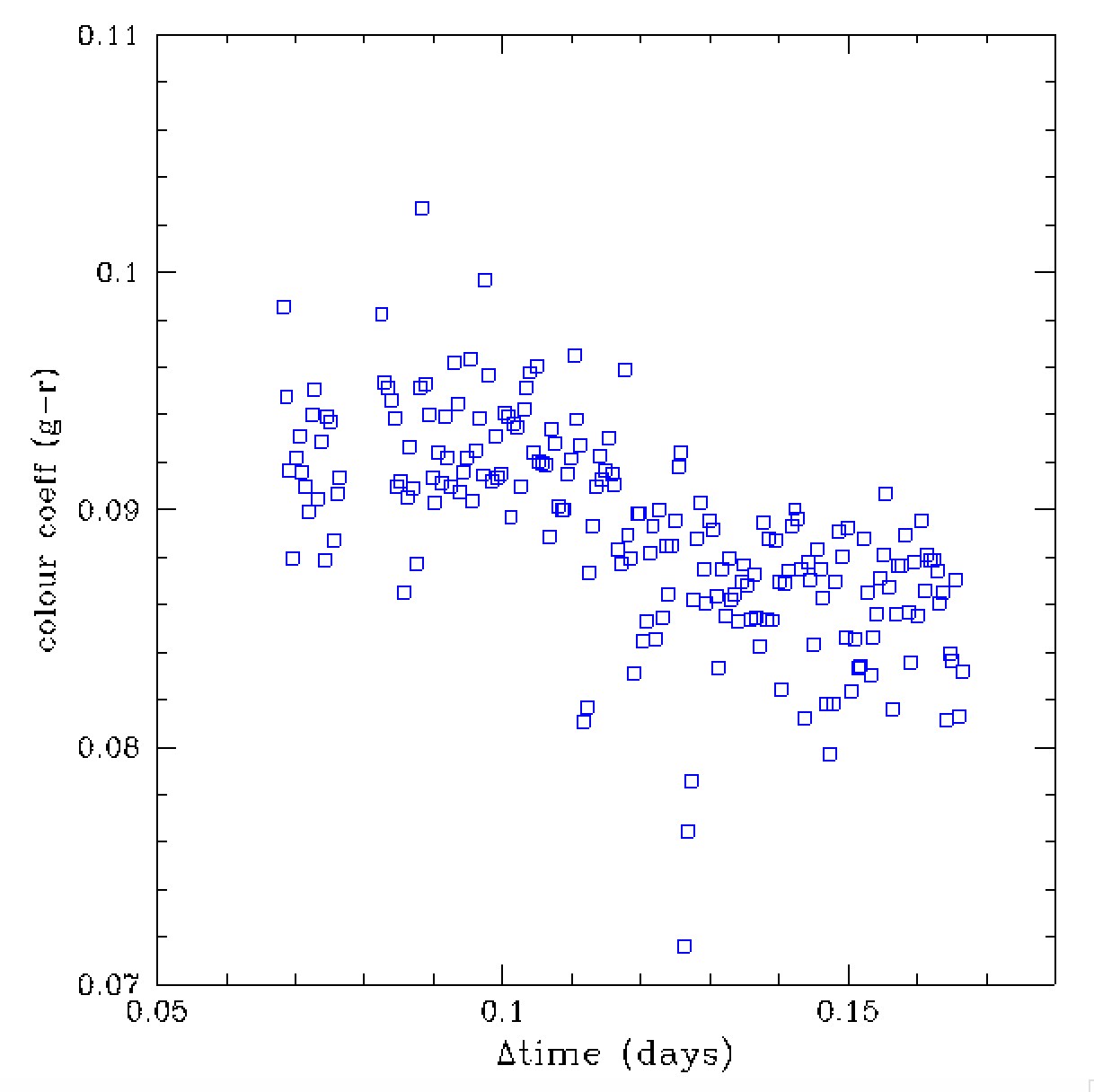
change in the image ZPs is seen to coinside with a slight change in colour
coefficents. Thus, the ZP change cannot be accounted by either airmass
variation or a single colour-dependent airmass variation.
Comparing this result with the prior plots above, this strongly suggests
that the transparency variation in this case could not be due to clouds alone.
Rather, another colour dependent atmospheric component, such as an aerosol
(Mie scattering), or water vapor (molecular absorption) must be present.
A change in air pressure could perhaps cause such a change since the
ZP difference is small only 0.05 mags.
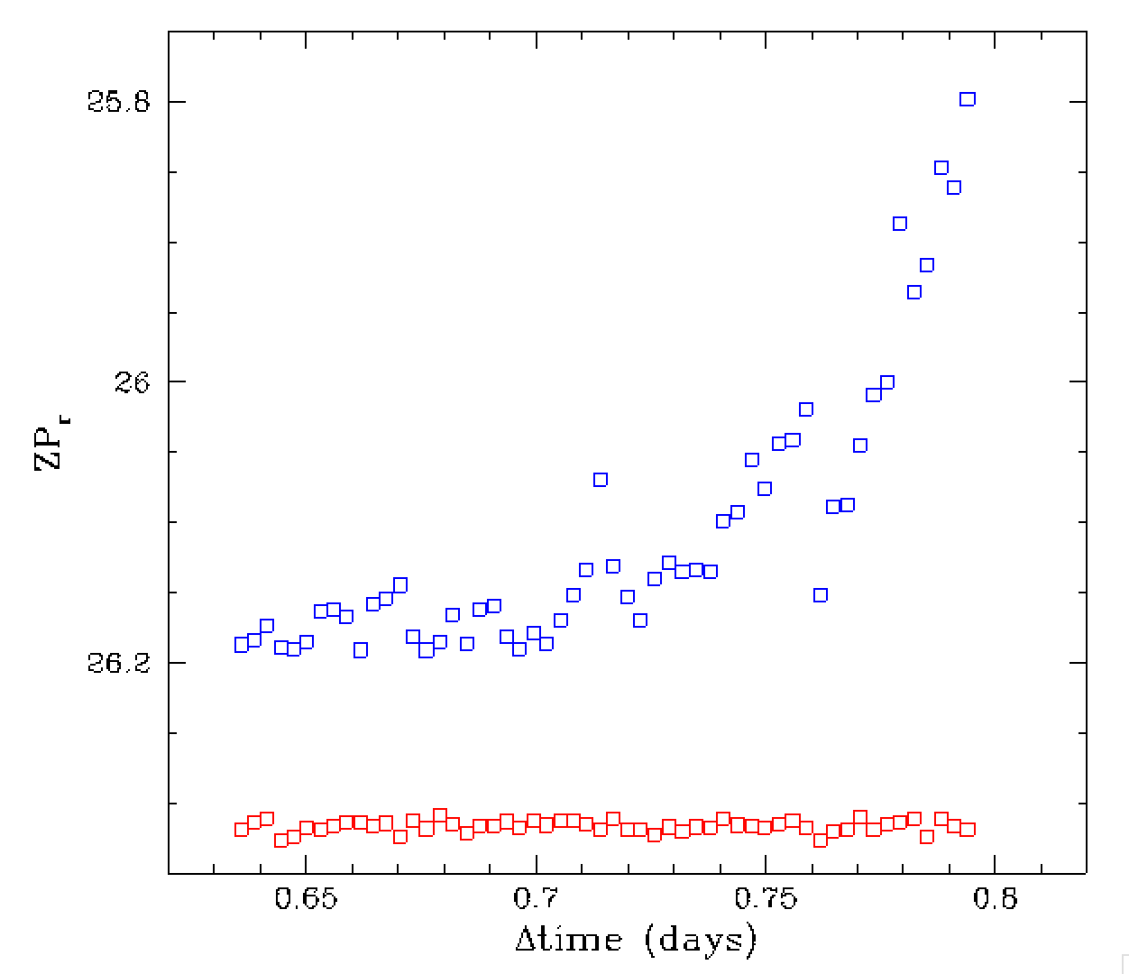
In the plot above we show the airmass corrected zero points for observations
of ZTF field 310 taken on 2018-12-22. Here we see relatively well behaved
data with a significantly disturbed region between 0.815 and 0.86 days.
In the plots above we show a sequence of three images for field 310 taken over
the span of a couple of minutes. Here we a discrete cloud enter and leave the
field-of-view. The colour coefficients in the previous plot suggest the
extinction due to this cloud is not purely gray as expected. However, the
interpretion is not completely clear since it is clear that not all of
the calibration stars will be extincted to the same extent. Thus, both
the ZP and colour coefficent are likely to be generally inaccurate.
In the plots above we show the zero points for a sequence of images of ZTF
fields 333 and 666. In the case of field 333 there were no obvious
discrete clouds seen in the images. Here the colour coefficients only vary slightly
compared to the prior example. However, extinction changes do correlate with
changes in colour to some degree. For field 666 there is no clear variation
in colour coefficents while the zero points varies significantly (suggesting
grey extinction).
In the above plot we see large variations in transparency that give rise
to a slight but clear variation the calibration colour coefficients.
Once the clouds pass the ZPs and colour coefficients become stable.
However, it is not clear when all of the cloud has passed since sources
on the edge of an image could still be effected without changing the
fit ZP and colour term.
In the plot above we show images corresponding to the calibrations given
above. Here we see the appearance of cloud causing a strong transparency
grandient across the image. The variation in ZP over the ~30 min
span between the two images is ~0.8 magnitudes. The most important point
to note here is that a single zero point or colour term cannot correct
for such transparency variations across an image.
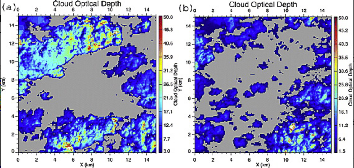
To consider more generally how complex the problem of transparency is with cloud,
below we plot the measured optical depth of thick (av. depth 14) cumulus clouds vs
thin cumulus clouds (av. depth 7). These figures are from
Wen et al. (2008).
From this plot we see that variations in optical depth of up to a factor of ~40
can occur across 0.5km. Assuming the average Palomar wind speed of
11km/hr,
we can expect to such changes over ~3 mins. So in such extreme cases, ZTF photometry would
vary by 4 magnitudes in Zp over ~5 ZTF exposures. Most cases are not this extreme.
The assumption made in prior Ubercalibation efforts by other surveys,
that transparency can generally be modelled as simple linear variation
during a night, appears to be fantasy. At Palomar such truly photometric
circumstances are likely valid for much less than half of the data.
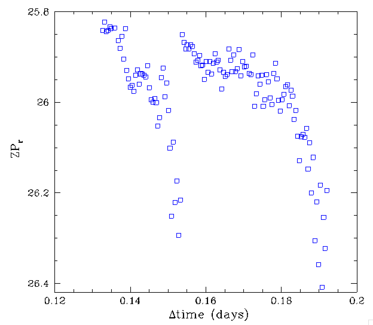
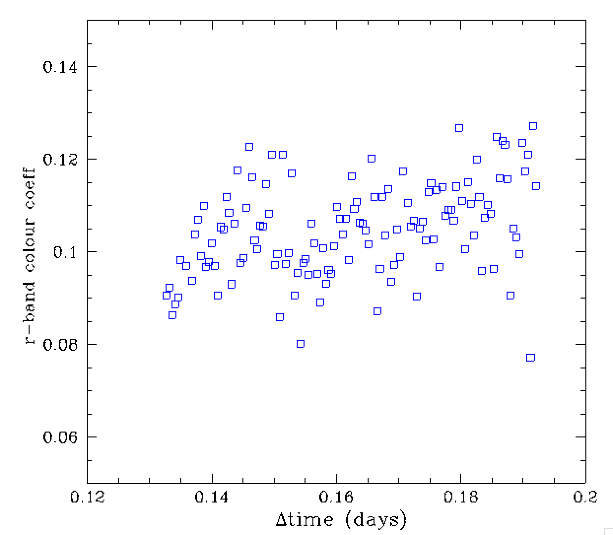
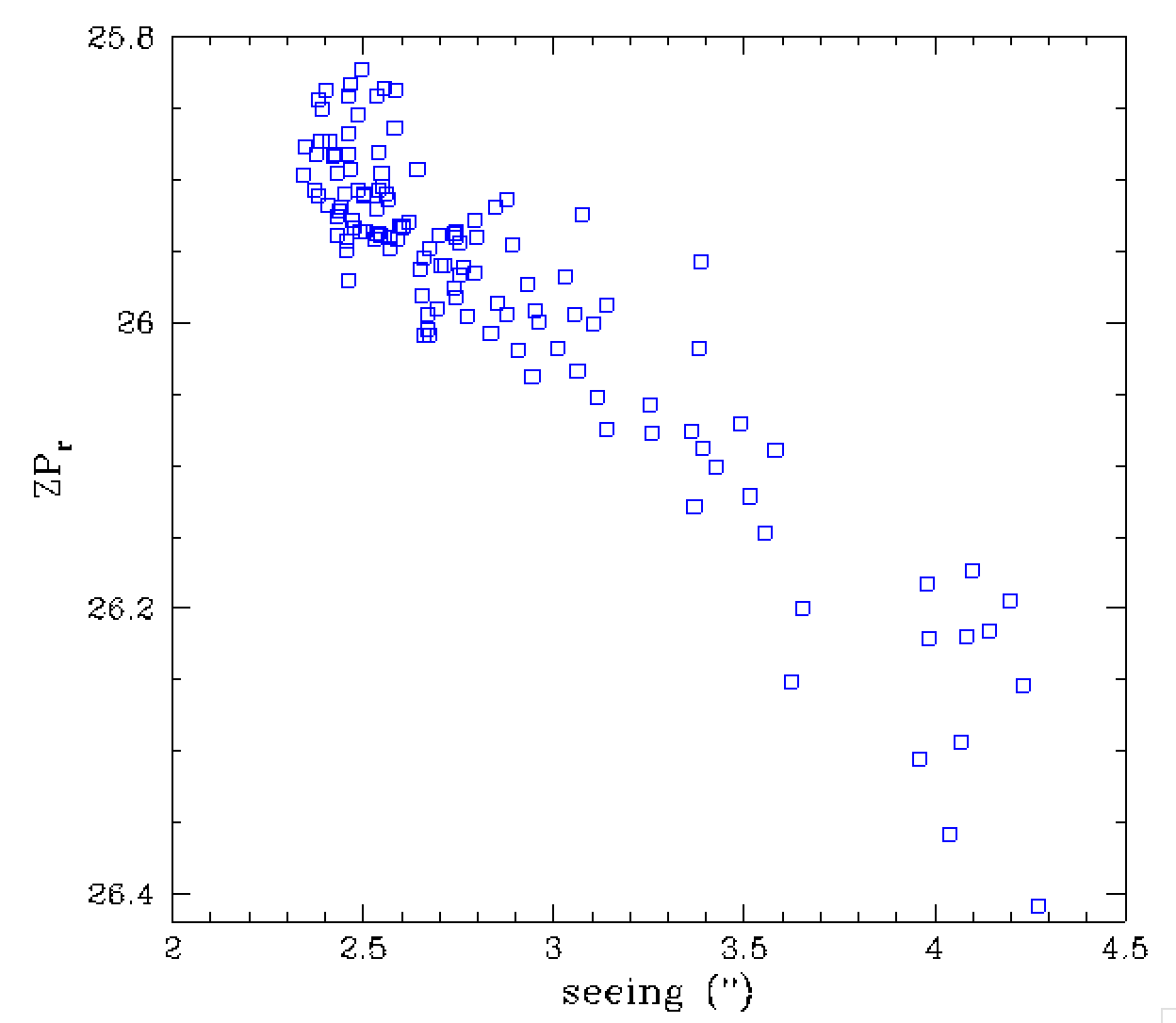
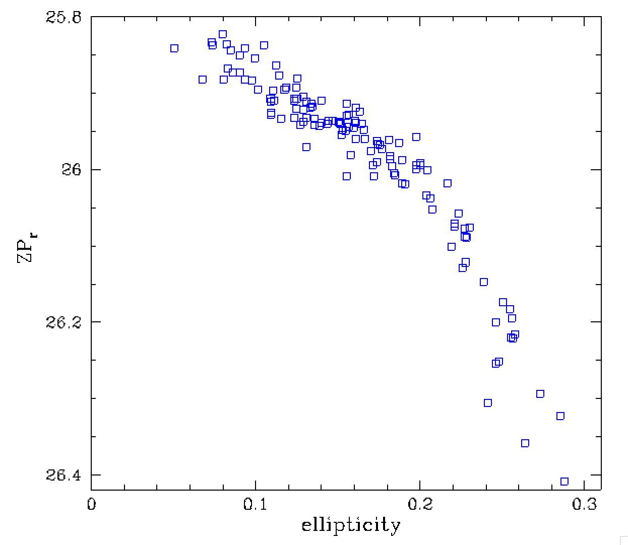
In the plots above we see a much more dramatic variation in zero point over
time for one night of observations of field 331. At the first the image
depth improves and then dramatically drops at around deltaT=0.15. In the
right image we see that any colour dependency of this change is uncertain
(suggestive of cloud). However, instead the bottom two plots show that the
depth is correlated with seeing and ellipicity. The most surpising point is
the depth increases with poorer seeing and greater ellipticity. This is
occurance is completely counterintuitive. However, here it is likely that the
photometry is actually bogus due the bad seeing in this very crowded field.
Thus changes in photometric zero points during a night cannot be account for
by transparency changes alone.
In this plot we see that, although there can be large variations in ZPs, due to cloud,
the variations in colour coefficents are typically relatively small (<~ 0.02),
This suggests that clouds that cause the major variations are gray.
Nevertheless, we can see that there is a trend at low levels of absorption.
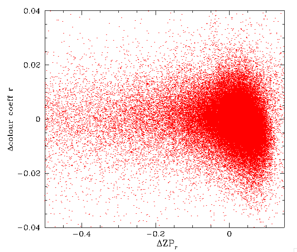
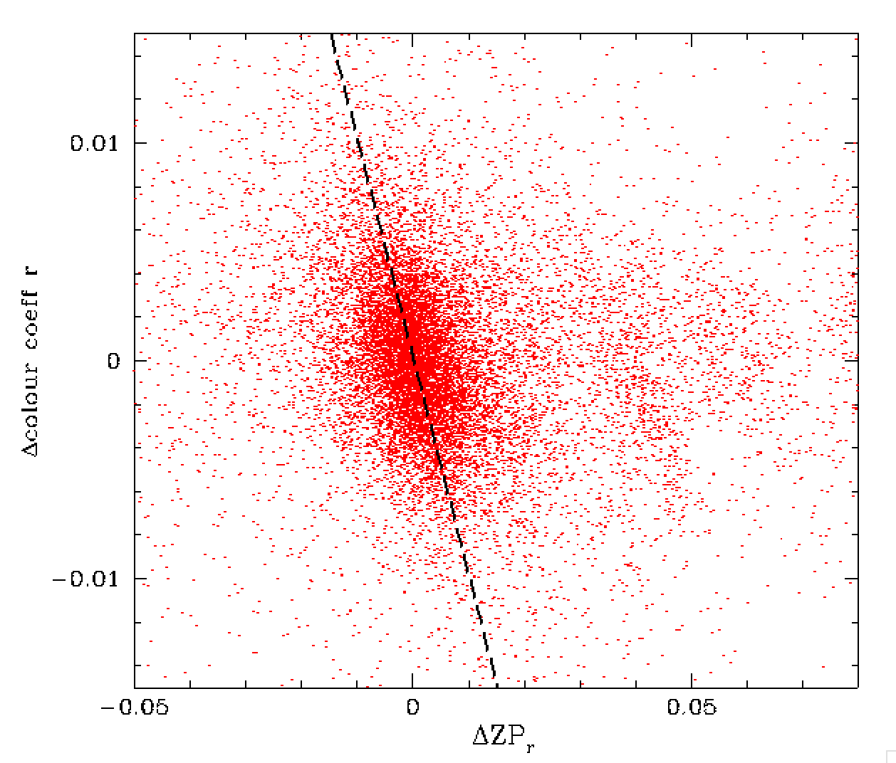
To get a better idea of atmospheric variations during a night, we take the values
from the 184 sequences of images taken on individual nights and subtract the
nightly average ZP and colour coefficient values from each.
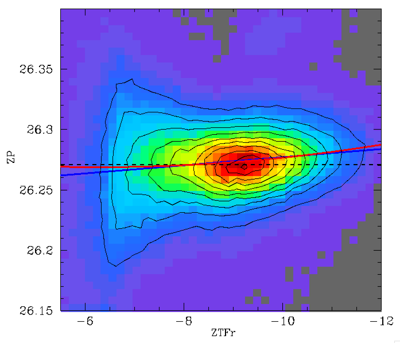
In the plot above see that there is indeed a clear variation in colour with
ZP. Here is this correlation is likely the combination of real variation in
colour with ZP along with correlated errors (since ZP and colour coeff are
jointly fit). This figure also shows that the variation in ZP and colour
coefficient during the span of a few hours tends to be relatively small
(delZP < 0.04, delcoeff < 0.02), although some far larger values are seen
(as shown above).
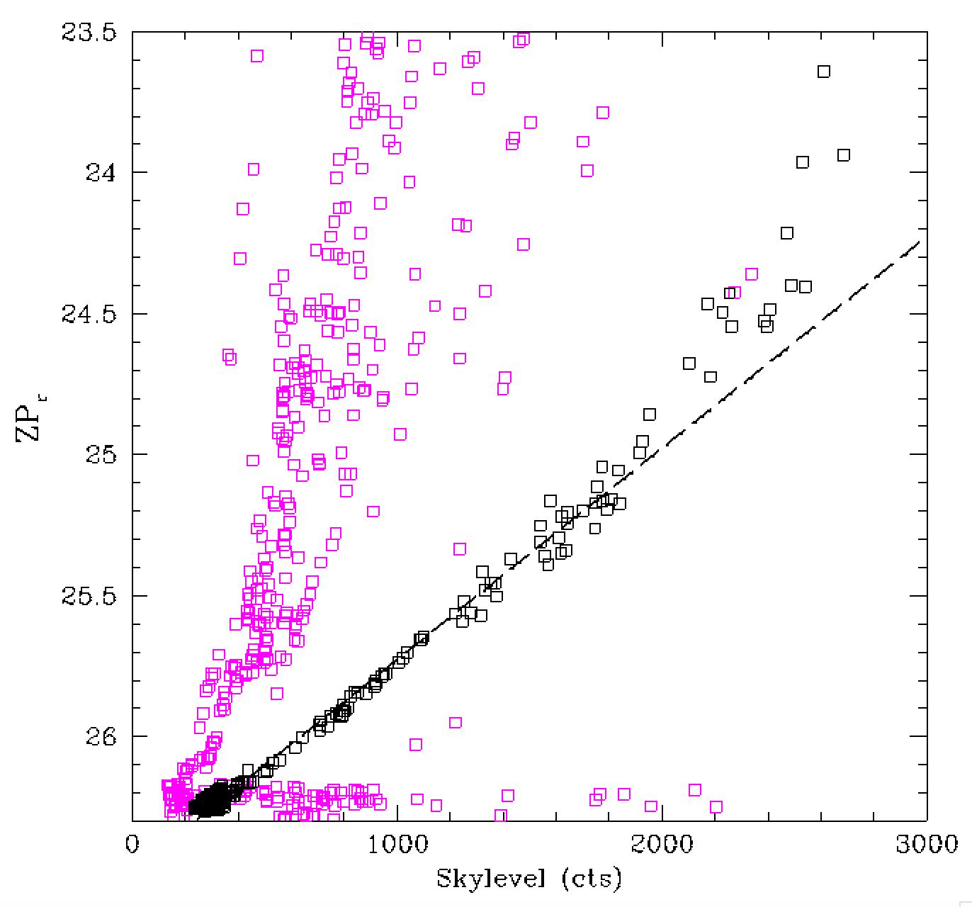
In the plot above we see that the decrease in zero point due to the clouds
in a field is well tracked by the change in background in that field.
However, as we noted above, the skylevel is dependent on lunar phase and
separation. As the righthand figure shows, the slope of the extinction
line varies between fields when multiple fields are observed within
a night, as well as between nights. Thus, on the bulk of nights, when
there is little lunar illumination, the skylevel cannot be used to
track extinction accurately.
However, based on i-band observations Zou et al. (2010, AJ, 140, 602)
suggest that the relationship between transparency and skylevel can
be determined based on the lunar phase function, lunar elevation,
and skylevel. They also note that only 50% of Gemini North observations
are photometric (extinction < 0.3 mags, <2% variation). Nevertheless,
the skylevel/transparency fits do not appear accurate beyond a 10% level.
In the above plots we show the results of Guyonnet et al.~(2019)
based on MERRA-2 atmospheric data (0.5 x 0.6 deg resolution).
From the above plot we see
that there is significant variation in transmission over time
with wavelength (particularly at CTIO).
The PWV nightly variations can range from 1 to 10% at the red
end where they would effect ZTF i-band observations. In r-band
(lambda < 750nm) the variations are up to ~2% within a night.
The PWV does not include liquid droplets in clouds. The
transmission model plotted above includes molecular O2
absorption which is important in r and i-band.
A large fraction of the transparency variation is attributed to aerosols.
These aerosol tracers include sea salt, dust, black carbon, organic carbon and
sulfate. This component is found to vary by >100mmag annually, and 10-20mmag
overnight. However, the uncertainties in the AOD (Aerosol optical depth) component are very large
(~22 mmag) and thus the MERRA-2 data is not ideal for determining transparency
at Palomar. A source of colour variation within g and r-band filters could
be due to O3 in the 500 to 700nm region (Chappuis band). However, this
component has a very small effect (<0.1% overnight) as shown above.
One possiblity for correcting transparency is to model a grid of
variations. Sky transparency can be modelled with MODTRAN, but this
costs thousands of dollars.
A possible alternative is lowtran.
However, this seems to be out of date and incomplete (see note on aerosols).
Another possibilty is LibTranRad.
This if free and has been compared to MODTRAN for LSST simulations and
found
to give very close results, except of i-band since O2 cannot be varied.
However, these simulations did not include aerosols (or clouds), which
are very important as noted above.
Tests of how well variations in airmass are modelled by standard photometric
fitting have been carried out by
(Stubbs et al. 2018) and show that linear and
quadratic airmasses terms used in fitting extinction are not ideal.
Zubercal tests
Due to the limitations of performing calibrations on a single image basis it
was decided to test the possiblity of calibrating full nights of data on
a quadrant or area. This approach is expected mitigate problems such as having too
few calibration stars in some fields/images. We also:
replace the g-r colour term with the more appropriate r-i (for r-band),
explicitly take into account source differential reddening wrt PS1 (which in r-band
is primarily responsible for the variation in the
colour term between fields),
explicitly take airmass into account (which is currently implicitly included in the
zero point determination),
explicitly include the colour term for the airmass-based extinction (which
is incompletely included in the current colour term determination).

The zero point and magnitude distribution for
the calibrated photometry. Left: data calibtrated with zero point,
Middle: data calibrated with ZP and colour coefficients.
Right: newly Zuber calibrated photometry.
Improving Zubercal
From the results above it is clear that more work is required to improve
the calibration beyond the current level. The data taken on 2020-04-29
contains many fields with differing extinction levels taken at differing
airmasses. These variations make it difficult to determine the source
of the time-resolved zero point varitions. To address this we selected
additional ZTF r-band photometry taken on 2020-11-13. This set contains
a couple of individual fields that were observed approximately
200 times in sequence during the night. Thus, we remove an possible
uncertainties due to differing reddening, crowding, pointing, etc.
The sole varations are due to airmass and transpancy variations.
With this data we initially concentrated on the r-band data taken
for fields 614 and 661.
Correlations between ZP and instrument data
In order to determine how much the physical factors affecting the
observations might also be affecting the photometry we investigated
corrlatations between the zero point variations and other observables
measured at the telescope. We determined the pearson and spearman
correlation coefficients between ZPs and temperature, humidity,
seeing, tip, tilt, wind speed, wind direction, and focus.
We discovered that, although the seeing was strongly correlated
with the values of tip and tilt (as expected), the zero point
variations were not correlated with the seeing or most of the
other parameters.
Including Chi and Sharpness parameters
As our prior
work
had suggested that the PSF fit quality parameters chi and sharpness were related
to photometric residuals, the next step was test how including this information
in the calibration would improve the photometry.
Atmospheric Transparency
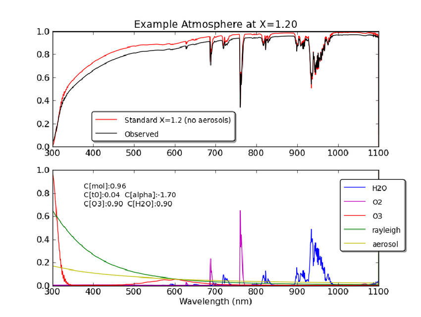
Wavelength dependency of the components of atmospheric extinction.
Left: extinction by component. Right top: combined transmission spectrum.
Right bottom: extinction model with the additional water and O2 components.
Mie (Aerosol) scattering vs Rayleigh scattering
The Importance of Transparency Variations
To consider how transparency variations might have affected our Zubercal
calibration we look variations in ZPs and colour coefficents in the current
individual frame calibrations.
A Broader Investigation of Transparency Variations
To better understand whether it is possible to model ZTF
transperancy variations during a single night we extracted
photometric zero points and colour terms for 91 fields that
had been observed in continuous sequences with > 50 images
taken on a single night. In some cases these fields were often
observed in sequences on multiple nights. So, in total this data
consisted 184 image sequences from single nights.
Conclusion
Considering all of the results above we can clearly say that varying atmospheric
conditions have effects on ZTF photometry that, in the absence of any
concurrent measurements with a photometric monitoring telescope
(as per SDSS, LSST, etc.), will be very difficult to correct to
a high level of accuracy. In fact, even separating bad data from
good data is a serious problem because ZPs that might be considered
OK data on one night, might signify data affected by variations in
transparency on another, since the baseline transparency level changes
from night to night. For example, r-band ZPs of > 26.1 suggest the
data is good. However, as seen from the plot above, rapidly vary
transparency is still seen in such data.
Other Sources of Rapid Photometric Variations
The Distribution of Nightly Photometric Variations
In order to get a better general idea of atmospheric transparency variations
we decided to look at how the individual measurements vary wrt the median.
We start by computing the changes in r-band ZPs and colour coefficents for
each observation of CCD0, quadrant 1, relative to the median values for a field.
Variation in ZP and colour coefficients relative to the median values.
Note, ZPs are corrected for variation with airmass.
Correcting Photometry for Transparency Variations
Historical Transparency Variations in Other Observatories
![]()
![]()