| Topics |
|---|
| Photometric fit parameter trends. |
| Photometric Zero point. |
| Colour Coefficient. |
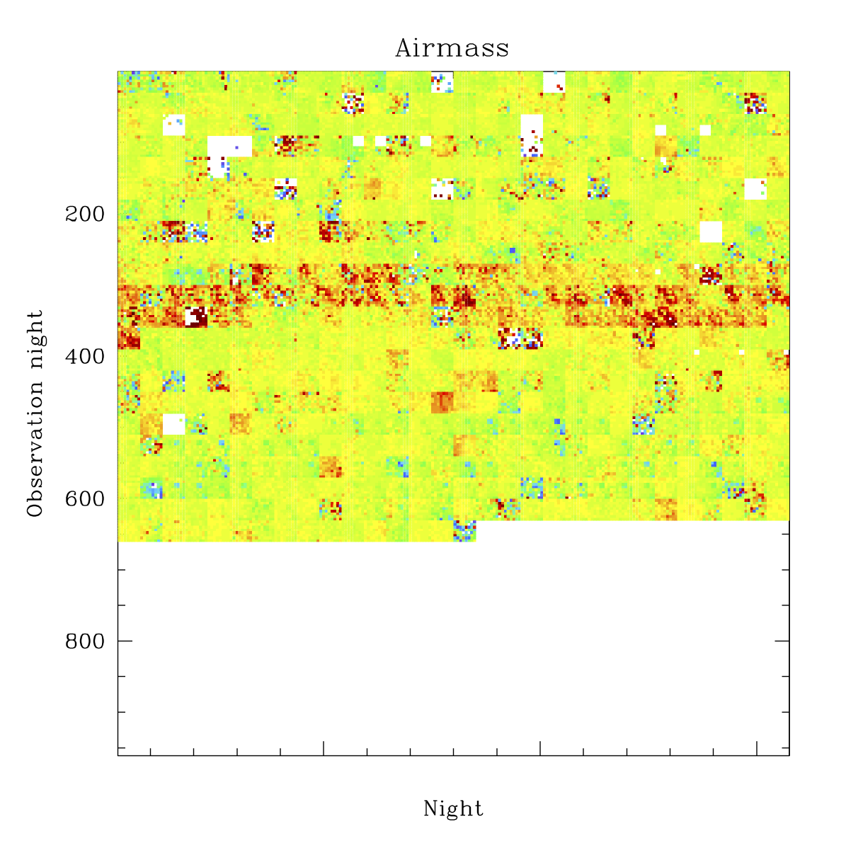
| Airmass. |
| Chi. |
| Sharpness. |
| Scale. |
| Importance of Lunar Phase. |
| Discussion. |
Trends in photometric fit parameters
Following our results from Zubercal calibration, we have started to investigate systematic trends in fit parameters. These parameters include zero point, colour coefficient, airmass, chi, sharp, and scale.The most important aspect here is perhaps how the parameters vary with time, since if the parameters were stable we would be able to hold them constant and potentially obtain more accurate fits. Similarly if the parameters vary in well defined way it could give better unstanding of the reson for the variation.
Zero point
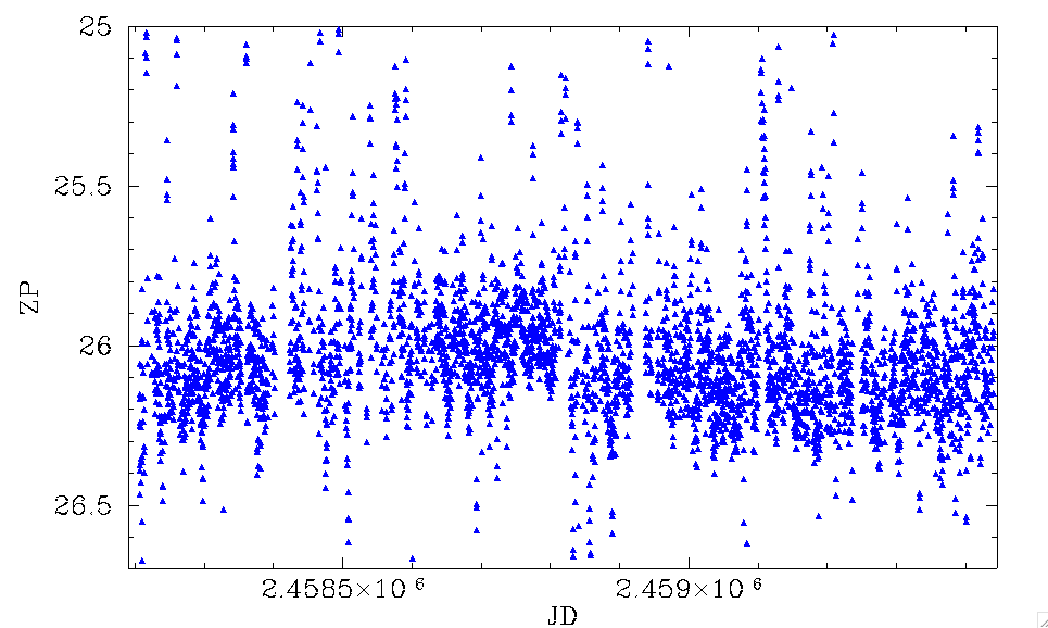
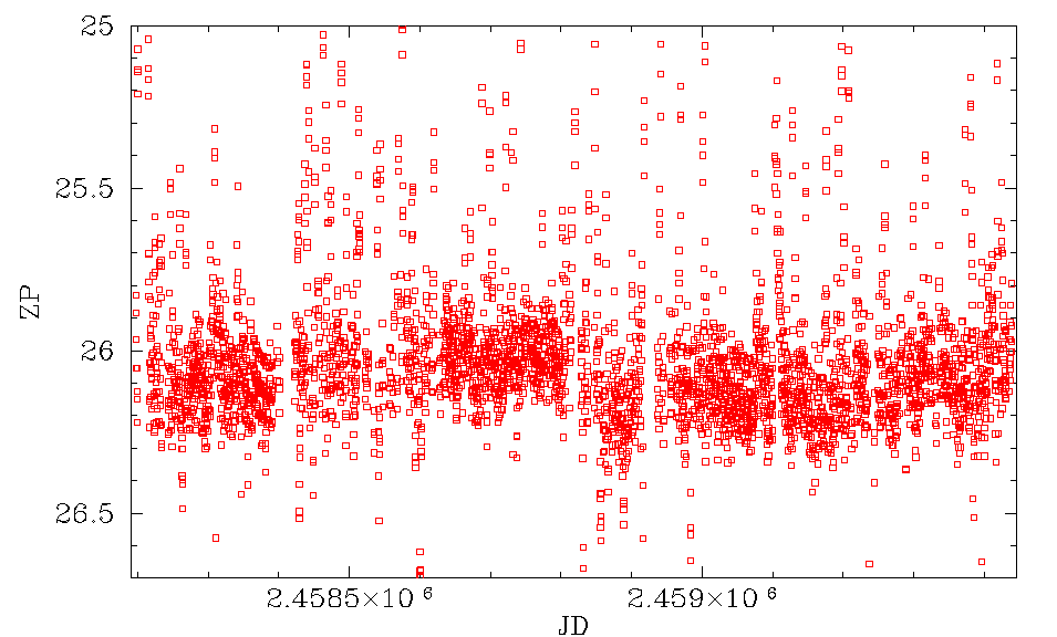
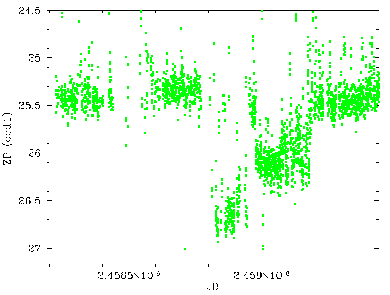
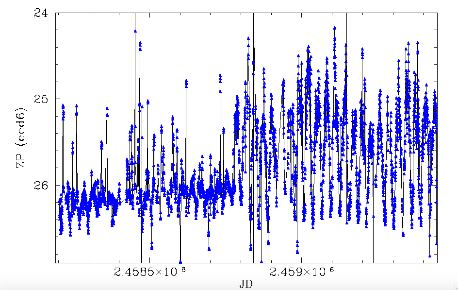
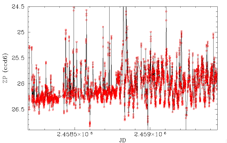
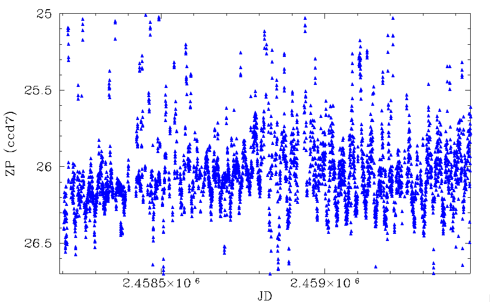
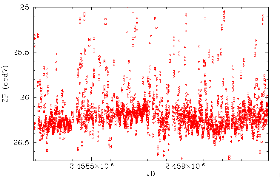
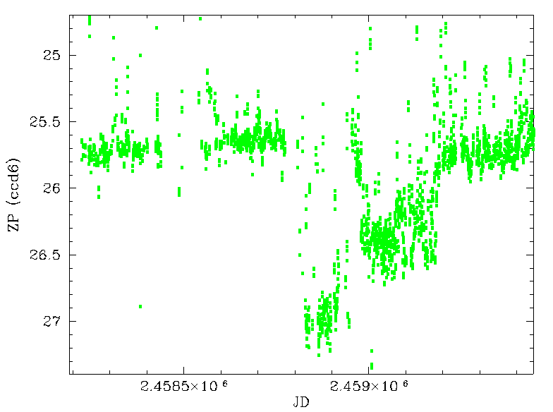
Variation in ZP with time for ZTF g, r and i band (blue,red,green). Top row CCD1, middle row CCD6, bottom row CCD 7.
In the plots above we show how ZP vries over time for three CCDs. CCD1 is a corner chip, CCD 6 is a badly behaved CCD near the middle, and CCD 7 is well behaved CCD. In the g and r-band data we see a long timescale modulation in the data with a timescale of more than a year. This may be related to long timescale weather patterns. The i-band has vary depth since long exposures were used for a couple of programs.
With the CCD-6 data we clearly see the monthly variation. This variation is largest in g-band and get much larger when the issues with CCD-6 began. This plot shows that the affect costs us more than 0.5 mags of depth in g-band on average.
In the CCD-7 data we see the same monthly variation but it is smaller than for CCD-6.
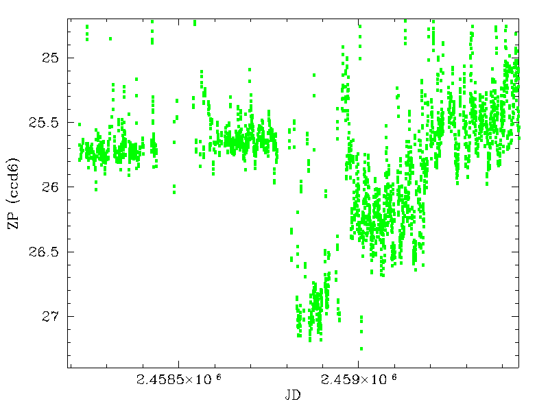
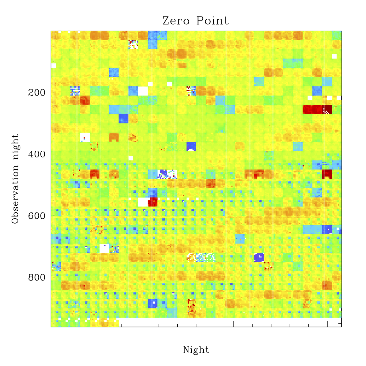
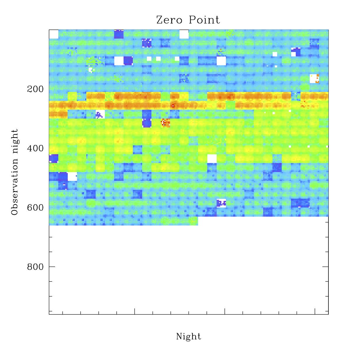
To get a better idea how each of the 64 quadrants varies over time we produce maps for the ZPs for each night.
 |
|
In the plots above we show how the ZP varies over time for all quadrants. White points are missing data or values outside of the range. As expected we see the circular vignetting pattern with deeper observations towards the center of the camera. The plot also shows how bad decreases the average ZP on a night and that some nights are deeper (due to long observation times). What we also see is how CCD-6 start deviating from the other CCDs midway through that data. Also, all of the data becomes strongly dependent on the lunar phase, not just CCD-6.
 |
 |
 |
|
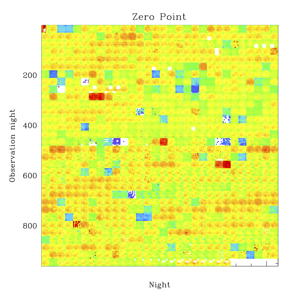
In the plot above we see the same kind of ZP valiations on some nights due to cloud or longer exposures. However, variations between individual CCDs is far less evident than in g-band. A small number of nights show instances where the depth of individual quadrants varies from the other CCDs. These results are probably due to fit errors and should be flagged.
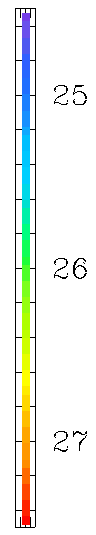
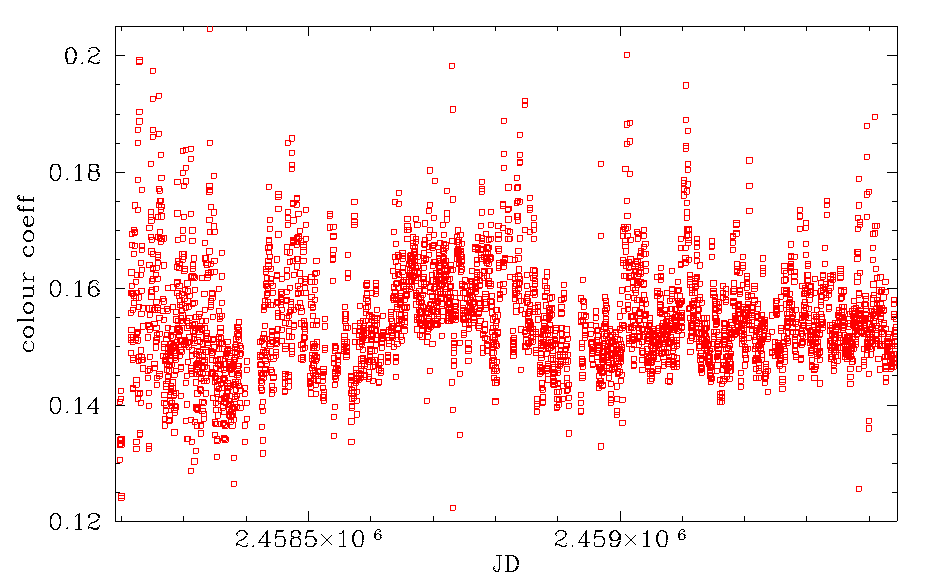
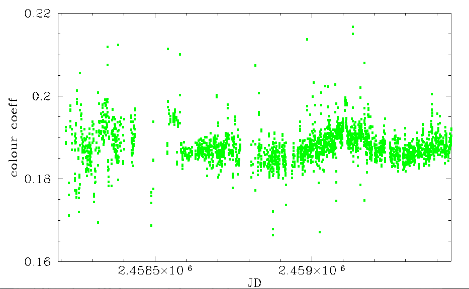
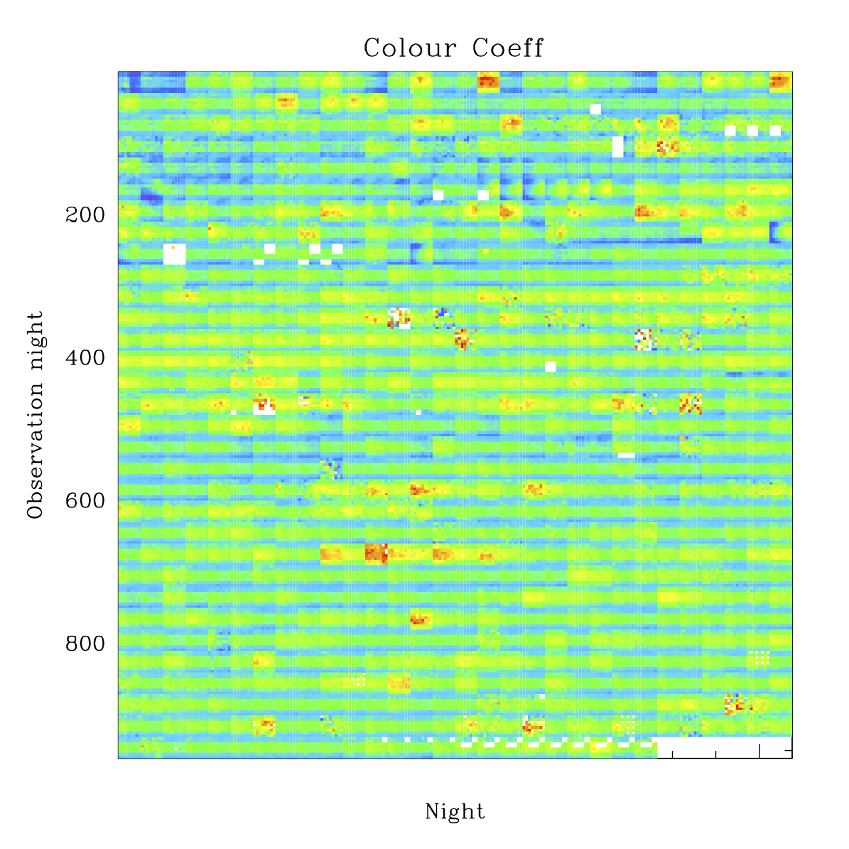
Colour Coefficients
As with the zero point we check for variation in the colour coefficient terms.
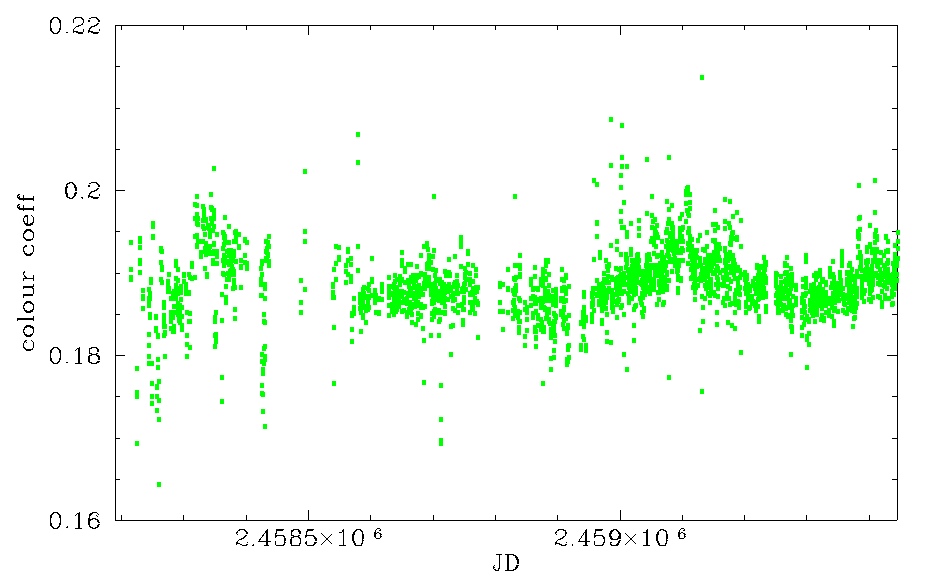
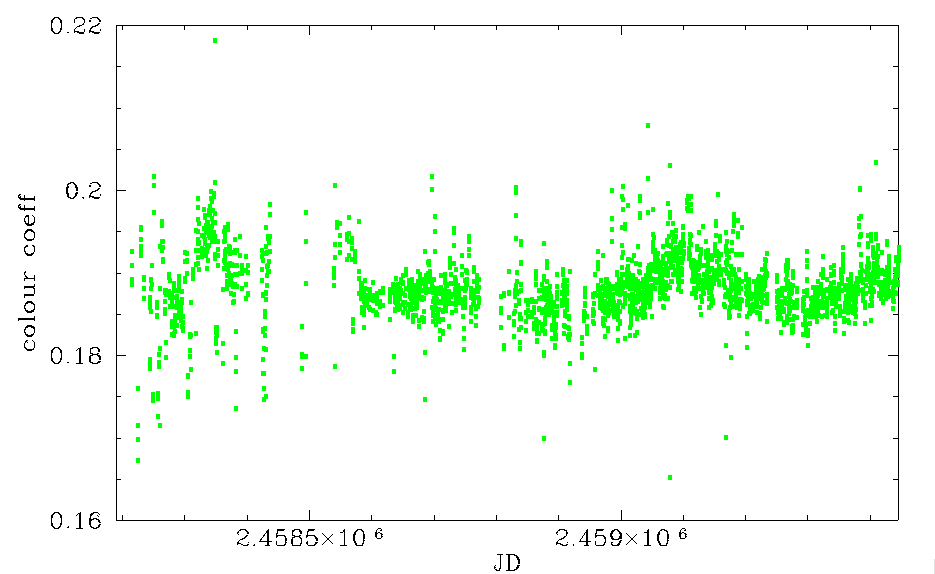
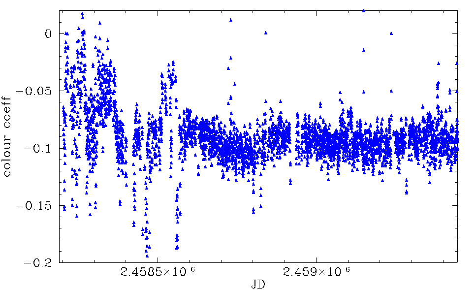
Variation in Colour coefficients with time for ZTF g, r and i band (blue,red,green). Top row CCD1, middle row CCD6, bottom row CCD 7.
In the plot above we see that there is little difference between CCD-1,6 and 7. This suggests that the issues with CCD-6 are not wavelength dependent. However, in the g-band plots we see that there are significant variation in the early data that disappears. The timing of these variations is similar to the sudden variation in the PSF position angle measurements. This suggests that the early data had a different colour dependence. This may be because different LED combinations were used to produce flatfields. Thus the data had a different colour dependence. Also we know that there were significant issues with flatfields in the first 400 days that have never been fully explained.
In all bands there are variations with time which are possibly related to annual variations in weather that produce colour dependancy in extinction. That is to say, the different atmospheric components vary in a seasonal manner. It is hard to explain the differences between bands in any other way.
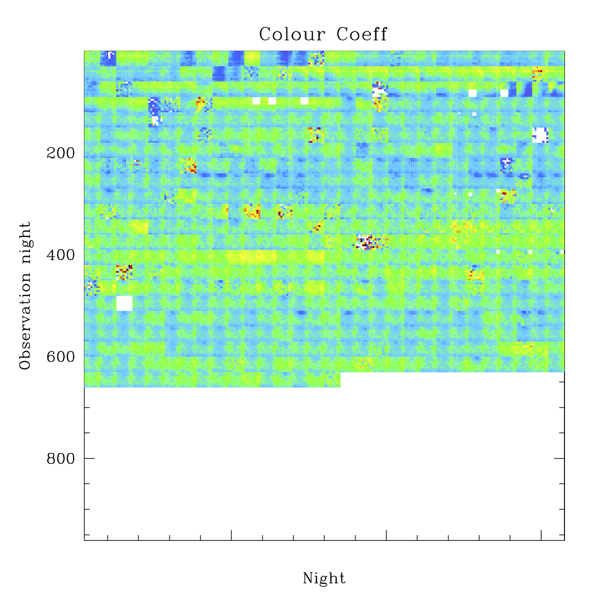
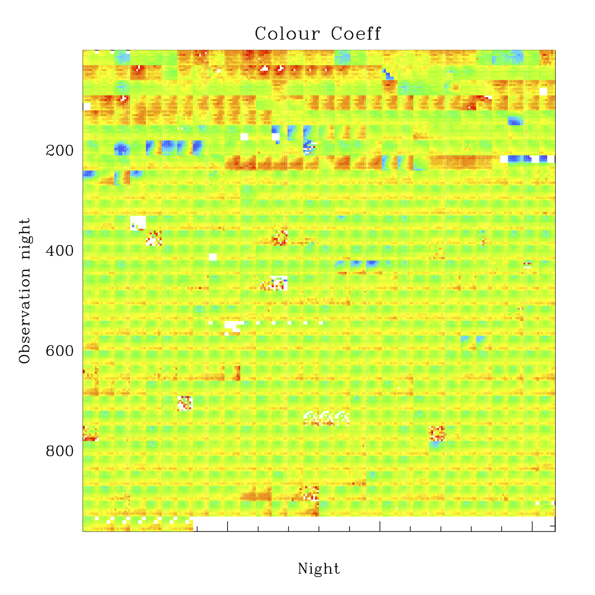 |
|
In the plot above we see that there are significant spatial variations in the colour coefficients in the early data. We expect different values for different quadrants. However, we do not expect variations in the structure from one night to the next. Thus, the reason for these trends is not at all clear. The more recent data is much more uniform but there still some nights that exhibit some variation across the camera.
 |
 |
 |
|
In the plot above we see that the r and i-band colour coefficients are show less variation with time. In r-band this variation seems mainly to be a scaling of the underlying structure due to the anti-reflection coating on the middle two rows of CCDs. In i-band the variations seem to be mainly seasonal.
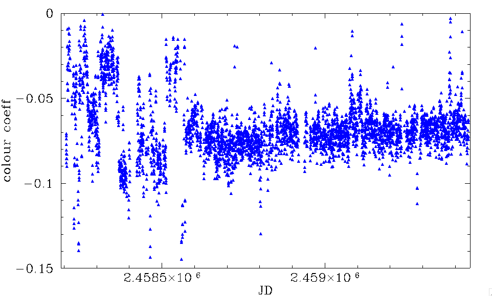
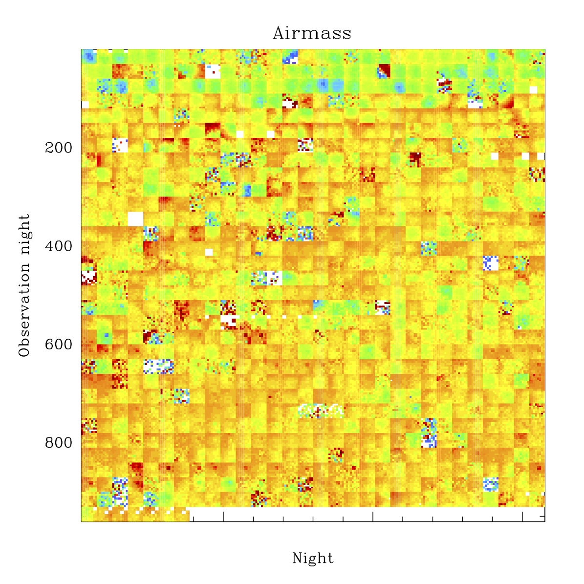
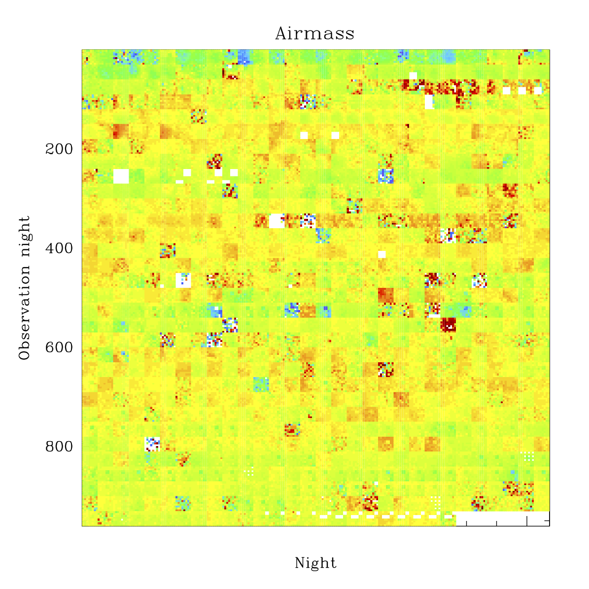
Airmass
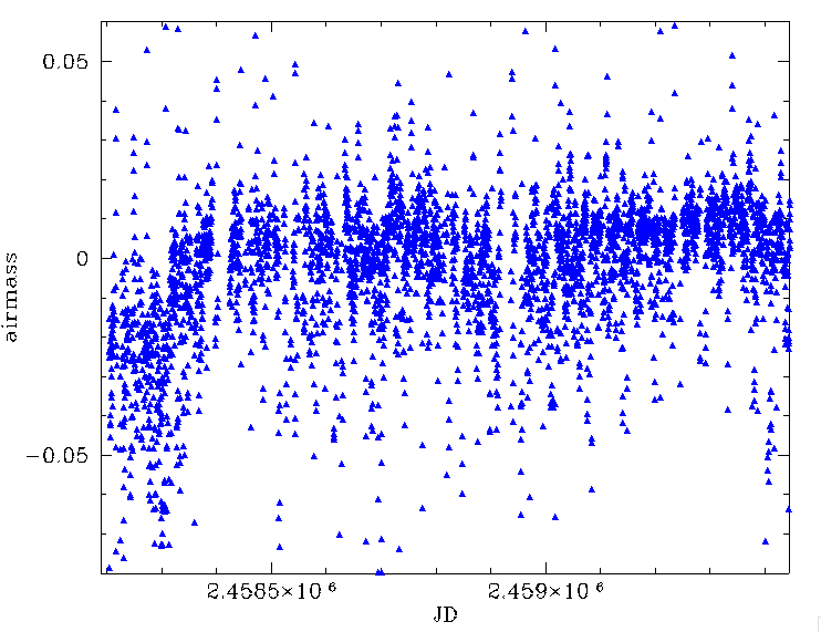
In our initial selection work we found clear dependence of photometric zero points on airmass. This dependency with later refined during our zero point modelling where we were able to predict zero points to 1.0%. The airmass effect itself is strongest in ZTF g-band due to the wavelength dependence to transparency.
|
In the plots above we can see that the airmass coefficients are vary significent with time and are centered near zero. This is unrealistic since the coefficients should only be positive. The reason for these values is that individual frames have zero point offsets. So the individual frame extinction due to airmass is removed by the zero point offset.
In the r-band plot above we see that there is a strong sinusoidal annual trend (as shown by the solid line). This is most likely due to variations in atmospheric components. The i-band data seems to show a similar trend. The reason for the large change in i-band airmass coefficients is unclear.
 |
|
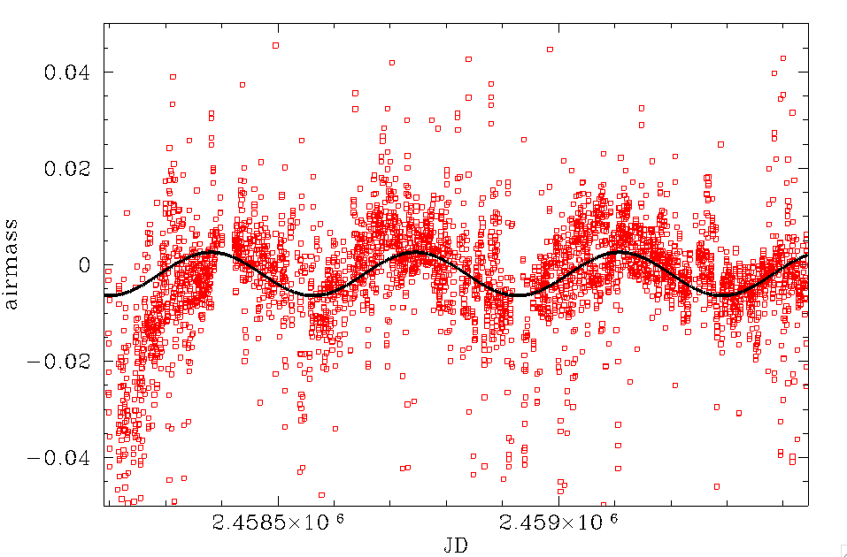
In the plot above we see that the g-band airmass coefficents are much more heterogeneous than the zero points or colour coefficients. Even on some nights there are significant variations between variations that are hard to reconcile. Nevertheless many nights show smooth contiguous spatial structure.
 |
 |
 |

|
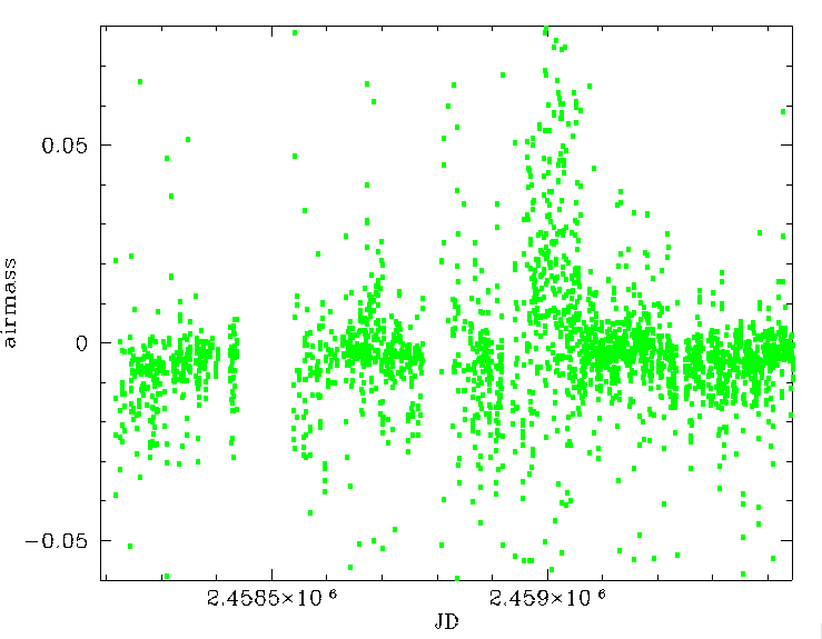
The r-band airmass coefficients appear to have a similar level of variation to the g-band ones. In i-band we see a period where the colour coefficients are significantly larger. These observations appear to match the period when long observations were taken. However, they do not match the earlier time when much longer observations were taken. The cause of this is unclear.
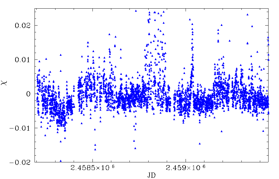
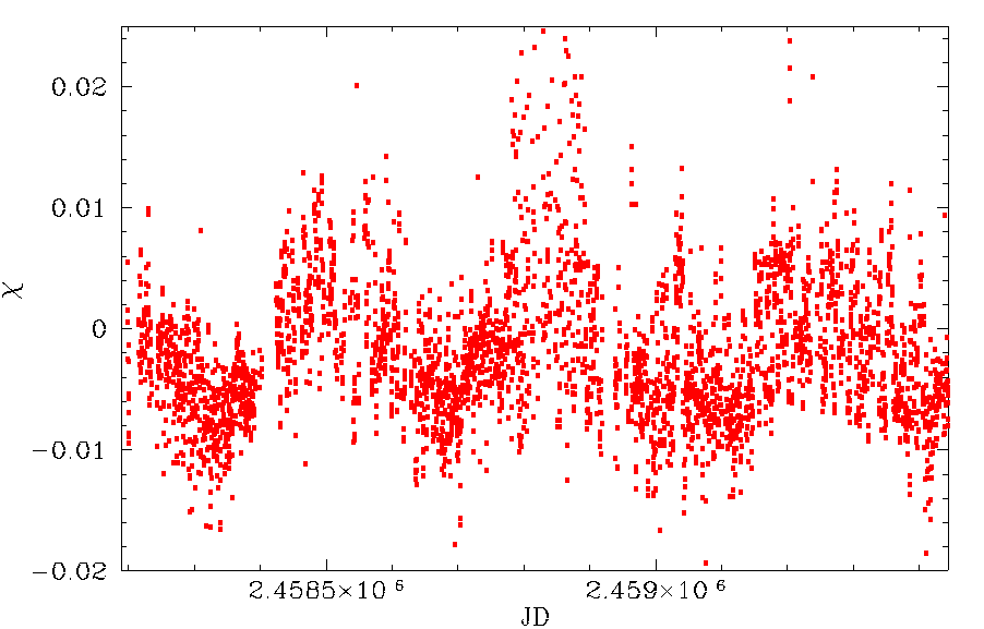
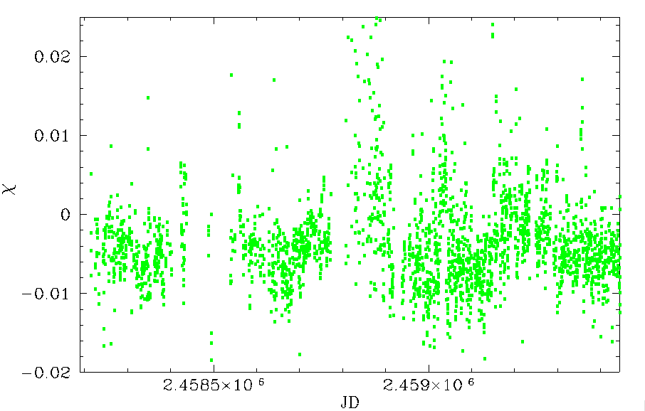
Chi
As we found earlier, inclusion of PSF shape parameters Chi (PSF fit residual RMS / expected RMS) and Sharpness (FWHM_obs^2 - FWHM_model^2) enable us to improve the ZTF photometry by taking into account spatial PSF variations. In particular, these PSF variations are reponsbile to the circular structures seen in individual ZTF CCDs.
|
I the plot above we see similar annual variation to the airmass trends. Interestingly the phase of the trend is different than the airmass. This is not unexpected since PSF shape is only partly related to observed airmass (i.e. differental refraction). Distortion of the PSF is affected by focus, tracking, as well as atmospheric turbulance. One expects that the last effect is related to weather (temperature/pressure/wind speed).
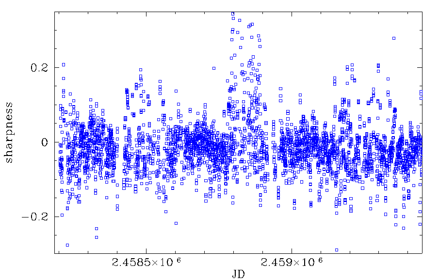
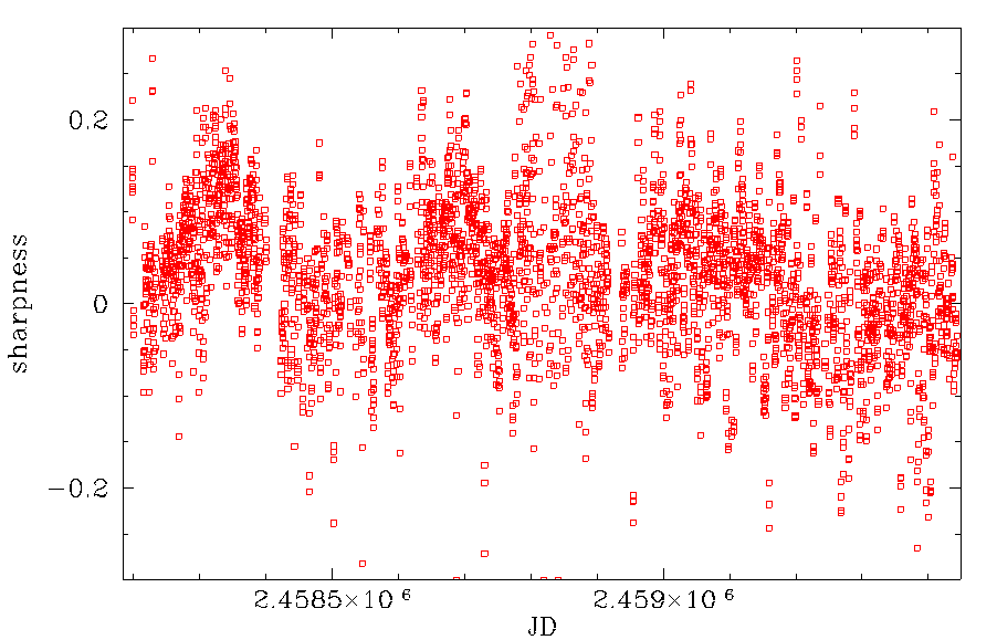
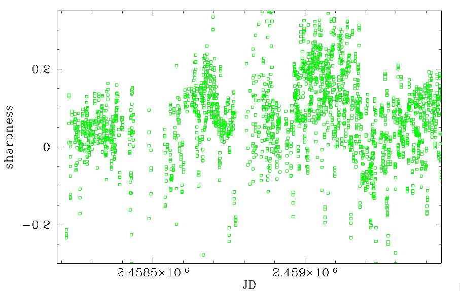
Sharpness
As with the Chi parameters, sharpness depends on PSF shape. Abrupt changes in sharpness are seen at the edges of the ZTF
|
As with the Chi plots we see modulations in the sharpness parameters that likely reflection seasonal variations in weather. However, the values are not as well correlated and the Chi values. Also, the variation in sharpness appear clearer in i-band unlike Chi.
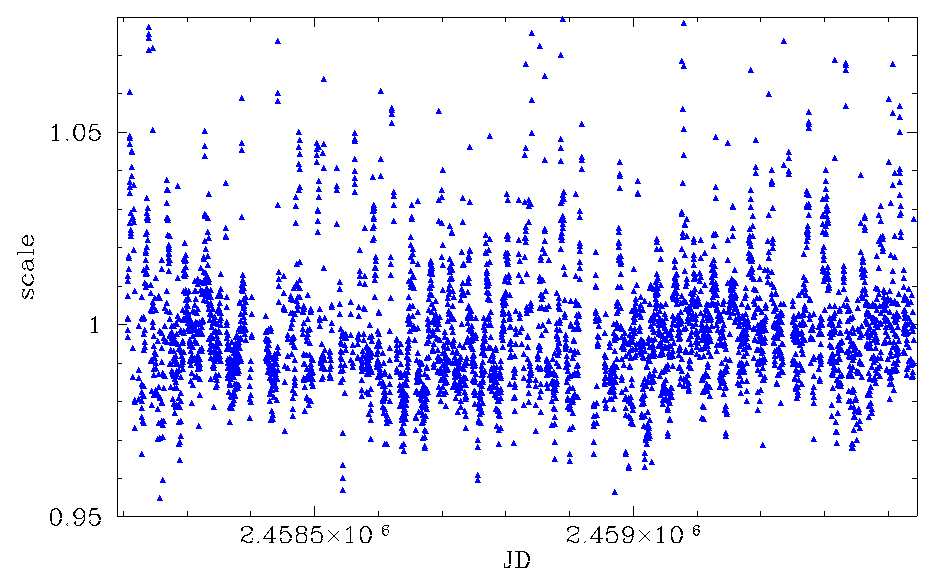
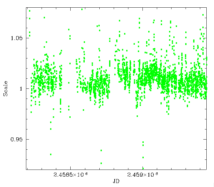
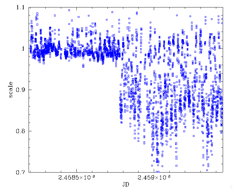
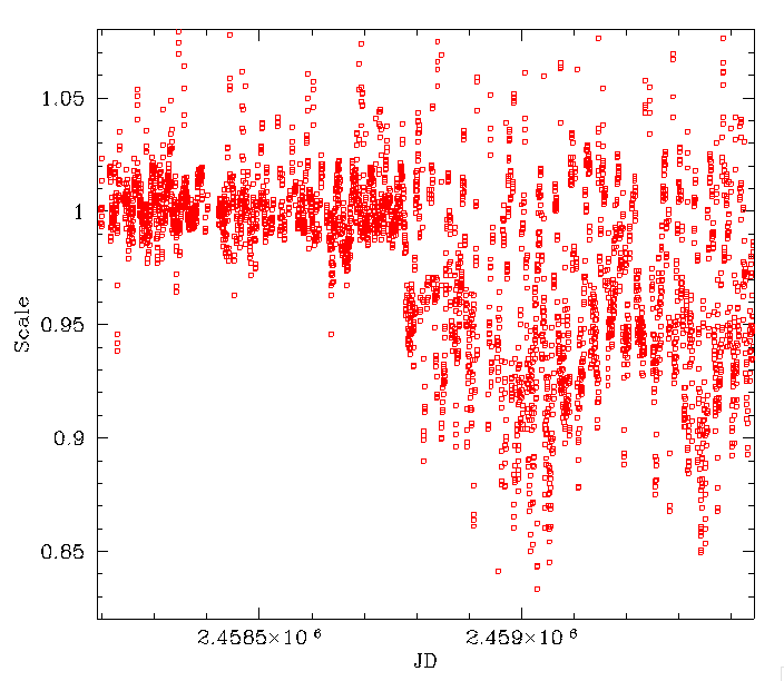
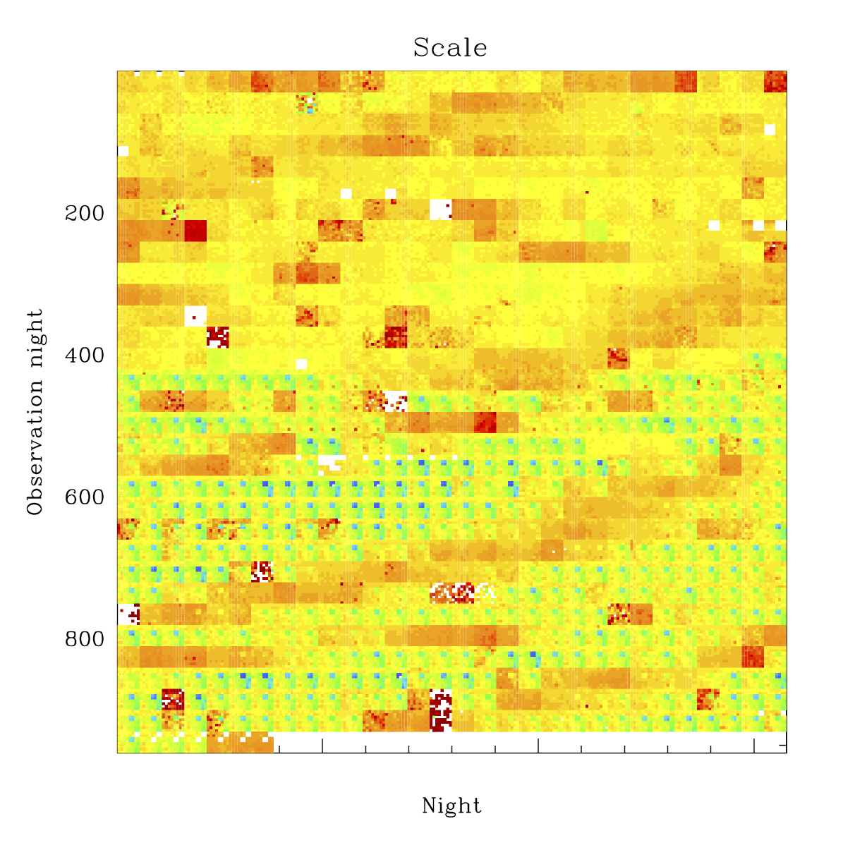
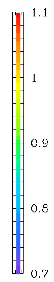
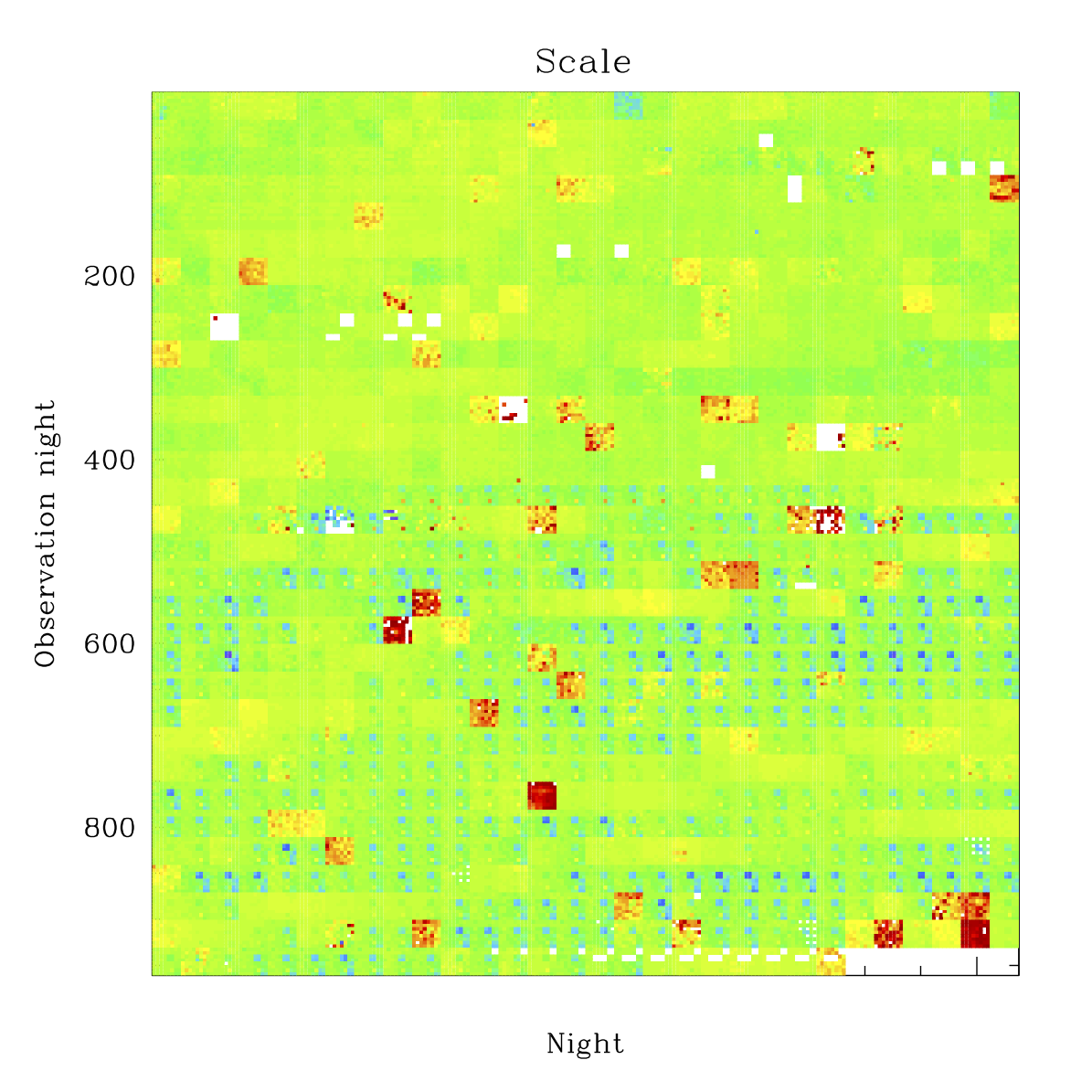
Scale
Due to the known issues with CCD-6 the Zubercal fit includes are scale term to account for a variation from the linearity not being 1.0.
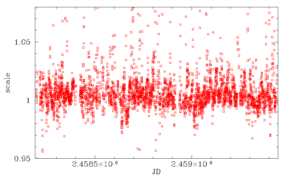
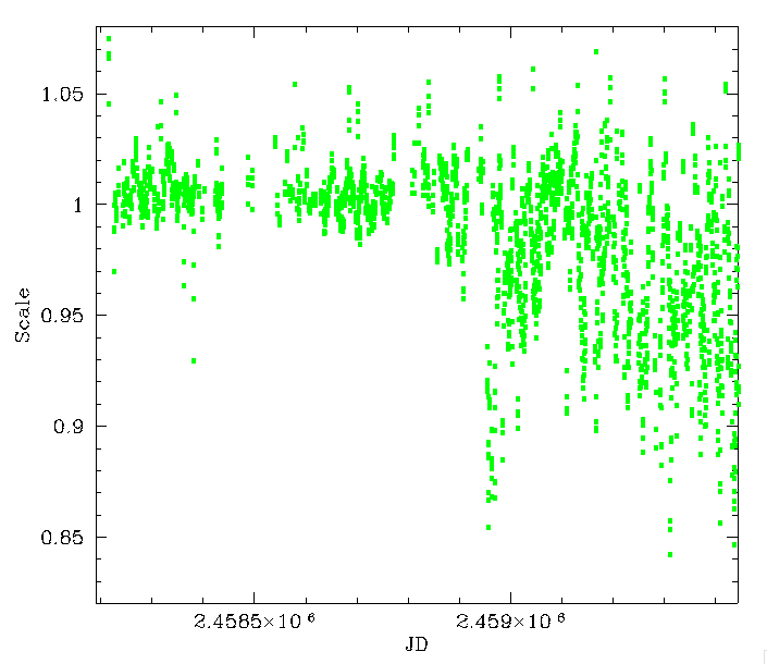
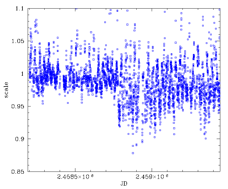
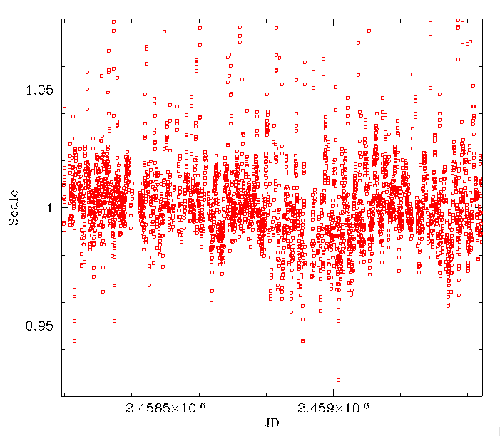
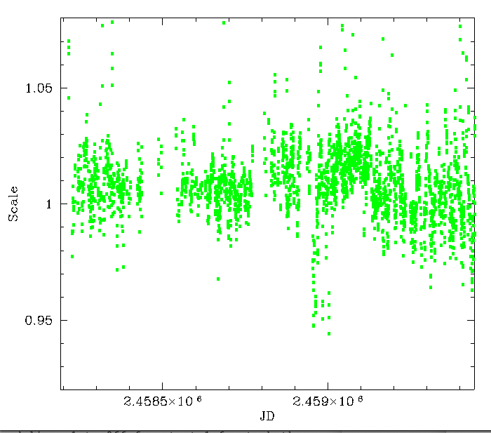
The ZTF g, r, i-band Scale fit coefficients over the span of observations for CCDs 1 (top), CCDs 6 (middle), and CCD-7 (bottom).
In the plot above we see that the scale in early data was generally close to 1.0 as expected. However, at later times the scaling can be seen to go wild for multiple CCDs. In fact, there are issues with CCDs 5,6,7,8,9,10,13 and 14. The issue is largest in g-band and is clearly present in r and i-band,
 |
|
In the plot above we see the spatial variation in the scaling factor for CCD-6. As we can see scaling varies with lunar phase. The CCD-6 data becomes consistent with other CCDs in bright moonlight conditions. The fact that other CCDs are offset is also clear.
 |
 |
 |
|
In the plot above we show the r and i-band scaling factors. The values are more conistent that g-band but also clear exhibit modulation in later data. There are also a few nights where the values are well offset from 1.0. These may be nights where there are only a few observations (so that the fits are not accurate).
Importance of Lunar Phase
To confirm that the observed variation in ZP above is related to the lunar phase of the observations (thus sky brightness), and changed significantly when the CCD readout process was changed. We divided the ZP data into two sets. Before and after the change in CCD readout waveform (on 2019-10-23). We then phase the data relative to the new moon on JD=2451550.1 and a synodic month (period = 29.530588853 days).
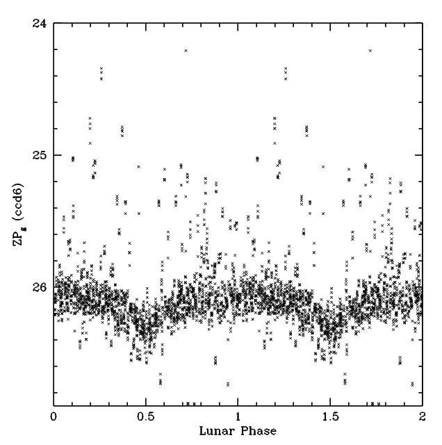
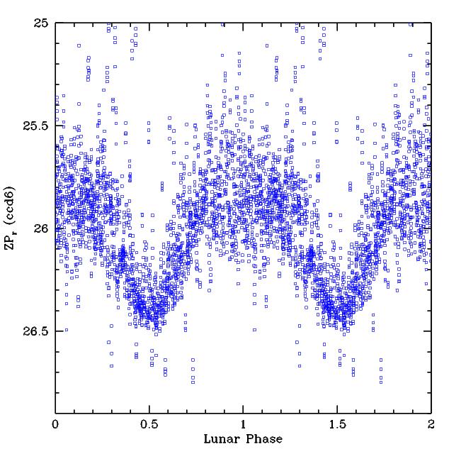
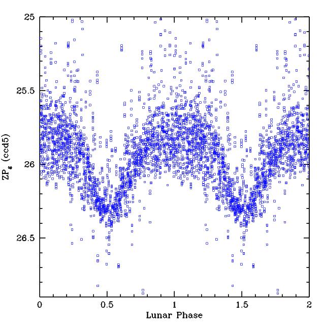
ZP varition with lunar phase relative to new moon (phase=0) for CCD6 in g (top) and r-band (bottom) for data taken before (left) and after (right) 2019-10-23.
Above we show the variations in photometric zero point with lunar phase. Here we clearly see that the effect is periodic with the lunar phase and that the affect is present in both g and r-band. We note that a smaller effect is present in the older data.
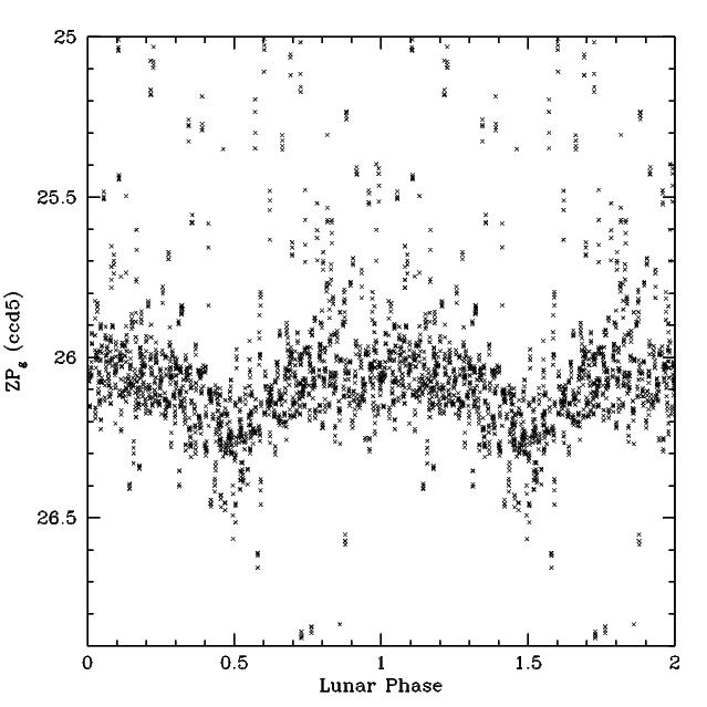
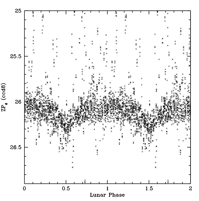
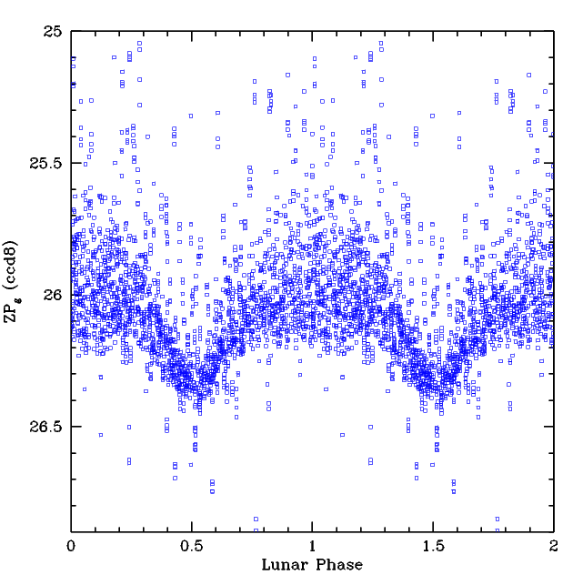

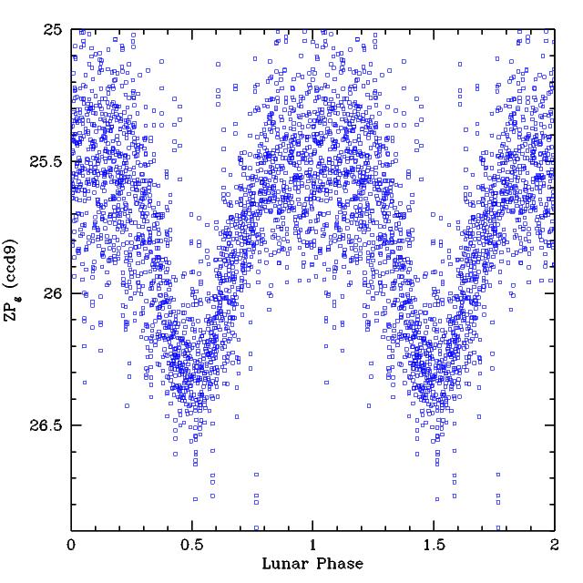
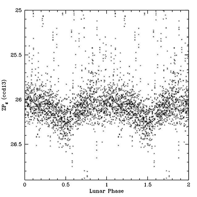
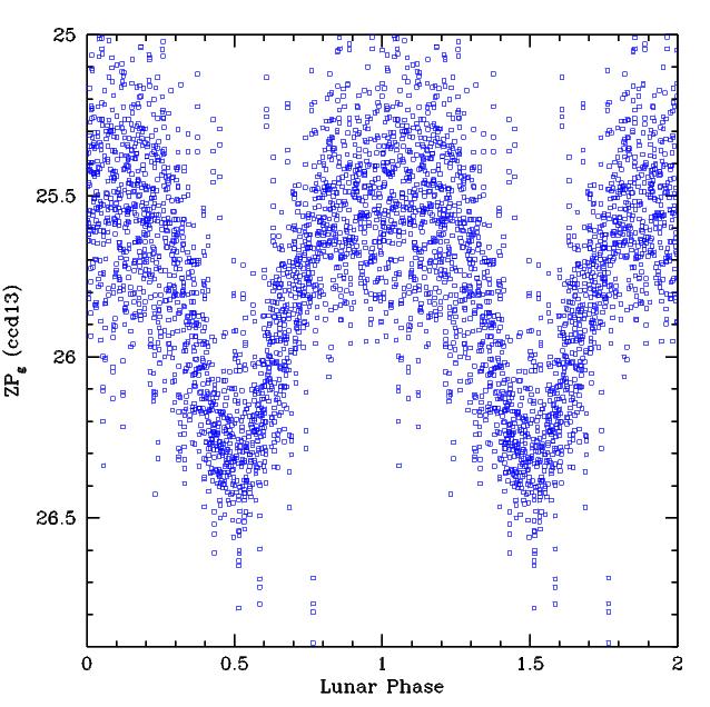
ZP varition with lunar phase relative to new moon in g-band for data taken before (left) and after (right) 2019-10-23. The plots are for CCDs 5,8,9, and 13 top to bottom, respectively.
To show that the effect is not just in CCD-6, above we plot the g-band variations for CCDs 5,8,9,13. Clearly the ZPs are systematically smaller near new moon counter to expectations. Additionally, although the affect is small in CCDs other than 6, it is present in most of the ZTF CCDs. Interestingly the amplitude of the effect varies a lot between CCDs.
Note, the variation in ZP with lunar phase is only clear in the Zubercal ZPs where there are scaling, airmass and other terms in calibration fit. In the original ZTF calibration process, the colour coefficient absorbs some of the variation. The true amplitude and origin of this affect is unclear.
Discussion
We have analysed the parameters of the Zubercal fits to ZTF g,r and i-band photometry. In almost every parameter we see strong trends with time.For zero points there is a long term trend lasting many years that might indicate long term weather variations (e.g. El Niño, La Niña). There also clear monthly variations due to sky brightness variations. These trends are very strong for CCD-6 and are costing ZTF more than 0.5 mags of depth relative to earlier observations. The monthly trends are strongest in g-band, but are present in all bands and all CCDs. In i-band there are strong ZP trends that reflect long exposure times used at various times.
For the colour coefficients we see different trends that are likely link to annual variations in atmospheric components. Further evidence for this comes for the variation in phase between different filter bands. Early observations show wildly varying coeffs as well as strong spatial structure. The reason for these trends is unclear, but suggests that the earlier data probably has lower quality. The effect is strongest in g-band.
The airmass coefficients are found to vary from unphysical negative values to positive with a very clear annual frequency. These do not reflect the true airmass coefficents, but are residuals due to weather variations since the average frame based extinction (which include both airmass and transparency) is already removed in the ZP fit. Importantly they reflect the fact that airmass coefficients are not constant. A number of nights show significant difference between quadrants. Such variations appear suspect. There are also some variations in i-band data that do not have a clear origin.
As with the airmass values, the chi and sharpness PSF parameters show annual trends. This is expected since varying atmostpheric components will cause variations in colour which in turn changes the PSF shape. Additionally annual variations in temperature and pressure will change the PSF shape. The phase of the peak in these trends is different than the peak of the airmass coefficients.
In our Zubercal process we introduced a scaling factor to account for the observed change in linearity after 2019-10-23 when the sky background was low. Here we see that the scale values are very far from the nominal 1.0 in many CCDs and most recent data. CCD-6 is the worst case, but CCDs 5,7,8,9,10,13 and 14 also show the a scale change that depends on lunar phase.