| Topics |
|---|
| Spatial structure in individual frames. |
| Complex Spatial Residuals. |
| Comparing Surface Fits in Complex Cases. |
| Towards Better Surface Fits. |
| Validation of RBF fits. |
| Discussion. |
Spatial Residuals within Individual Frames
After correcting ZTF frame photometry for the average spatial residuals. and the dependence on colour we determined the residual scatter. We compared this to the scatter in the current ZTF calibration. In almost all cases there is a slight improvement in the calibration based on the scatter relative to PS1. However, the amount of scatter was still seen to vary wildly from one night to the next. Since most of the underlying instrument variations have been corrected (no corrections are yet applied for the time dependence on spatial structure), the remaining residual can be attributed to external sources. The most obvious cause are variations in transparency due to clouds.Since the Zubercal calibration process itself iteratively corrects for average offsets between observations due to varying transparency, the variations must be on spatial scales smaller than a quadrant.
To see how the residuals varied within an individual frame we examined the residuals vs their image coordinates. As expected there are many cases where variations have a simple spatial dependence.


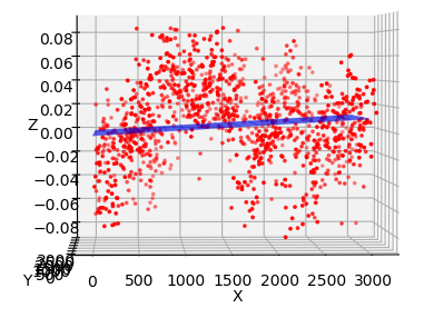
A g-band observation of ZTF field 858 (CCD-6, quadrant 1) taken on 2020-03-06 and the photometric residuals relative to PS1 after the initial Zubercal processing. The grid in the left plot represents a polynomial surface fit to the residual photometry.
In the plot above we see the presence of strong spatial residuals that are well modelled by simple polynomial fit (tilted plane). As we can see from the image the presence of a gradient in the residuals matches a gradient in the sky level (i.e. the attenuation by cloud is correlated with a higher skylevel in the image).
We expect a large fraction of the systematics in the residuals can be corrected by such a model. In more complex cases higher order fits are required. However, there are much more complex residuals that are very poorly modelled by such simple functions.
Complex Spatial Residuals


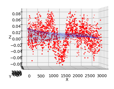
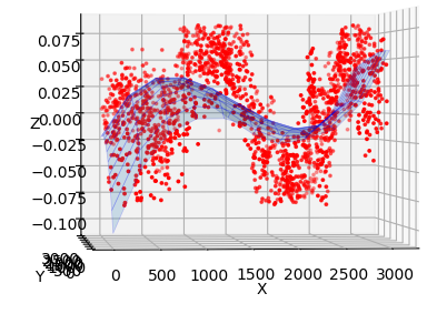
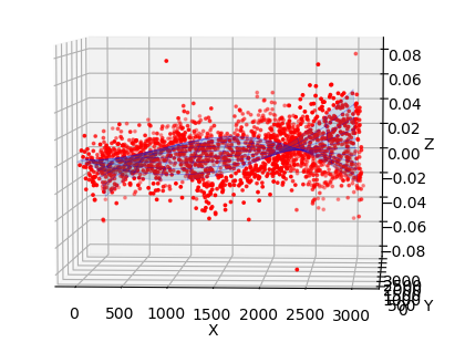
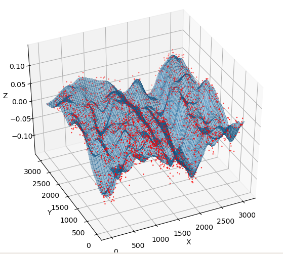
Spatial residuals in three r-band obsevation of ZTF field 592 taken on 2020-02-24 calibrated to PS1 for CCD-6 quadrant 1. The grid represents a polynomial surface fit to the data.
In the plots above we show how spatial residuals in three exposures of the same field observed over a span of 10 minutes. Clearly we see that there is strong spatially correlated and complex residuals. Since the residuals vary from one observation to the next we can say that the variation is not related to any incorrect calibration of the underlying average spatial structure (and it is very unlikely related to rapid instumental changes).
Additionally, we see that the polynomial surface fits are incapable of representing the underlying structure.

Spatial residuals in three r-band obsevation of ZTF field 592 taken on 2020-02-24 calibrated to PS1 for CCD-6 quadrant 2.
As a comparison to the residuals from quadrant 1, above, we plots the residual structure for quadrant 2.

The surface fits to the r-band residuals in the four quadrants of CCD6 for ZTF field 592 taken on 2020-02-24 calibrated to PS1.
In the plot above we show the fit surface combined from each of the four quadrants of CCD6. These fits correspond to the first exposure in the plots above.
Comparing Surface Fits in Complex Cases
Since the polynomial fits are incapable of represent the residual surface we add fits for Chebchev, Legendre and Hermite polynomials as well as splines.


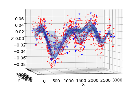
Spatial residuals and fits to r-band obsevation of ZTF field 592 taken on 2020-02-24 calibrated to PS1 for CCD-6 quadrant 1. The grid represents the surface fits to the data for fifth order Chebyshev, Legendre and spline fits, respicatively.
In the plots above we show a set of fits to the residual surface using different types of polynomials. As we can see all are essentially the same and none are very good. To properly fit the residuals a more complex surface model is required.
Towards Better Surface Fits
To see how different types of fits deal with complex cases we perform a series fits on every single frame. The most simple fit is a plane.


Spatial residuals and fits to r-band obsevations of ZTF field 592 taken on 2020-02-24 calibrated to PS1 for CCD-6 quadrant 1. The grid represents a plane fit to the data with the resulting residuals after this correction. The lower images show binned residuals to the data and the results.
In the plot above we show the residuals when a plane is fit to the residuals. Clearly there are significant residuals that remain after this correction.


Spatial residuals and fits to r-band obsevation of ZTF field 592 taken on 2020-02-24 calibrated to PS1 for CCD-6 quadrant 1. The grid represents the surface fits to the data for fifth order Chebyshev fit.
In the plot above we show a fifth order chebyshev polynomial fit to same data. Clearly there is a very significant improvement to fit as the scatter in plots show. However, this model is still does not accurately model the sitiation.
We fit the same data with a high order spline fit to the the data. However, spline functions perform very poorly in data that has gaps. The unconstrained fits diverge at such locations and are thus not useful at constraining the data. In order to improve this situation we created a spline fitting routine where points were added at points where the fits gave values that lie outside the bounds of the data. This process insures that the fit is better behaved. However, complex cases may poorly represent the true distribution of data.
Radial Basis Functions
An alternate to using splines is to use radial basis functions. These a functions that are centered on the locations of measurements and decline with distance in a uniform way. In the their unconstrained form, like high order spline fits, they are used to interpolate values and pass through every measured point. However, since real data is noisy, they poorly represent values away from the measurements (over fitting). However, as with spline it is possible to better respresent a lower order variation by smoothing the data.


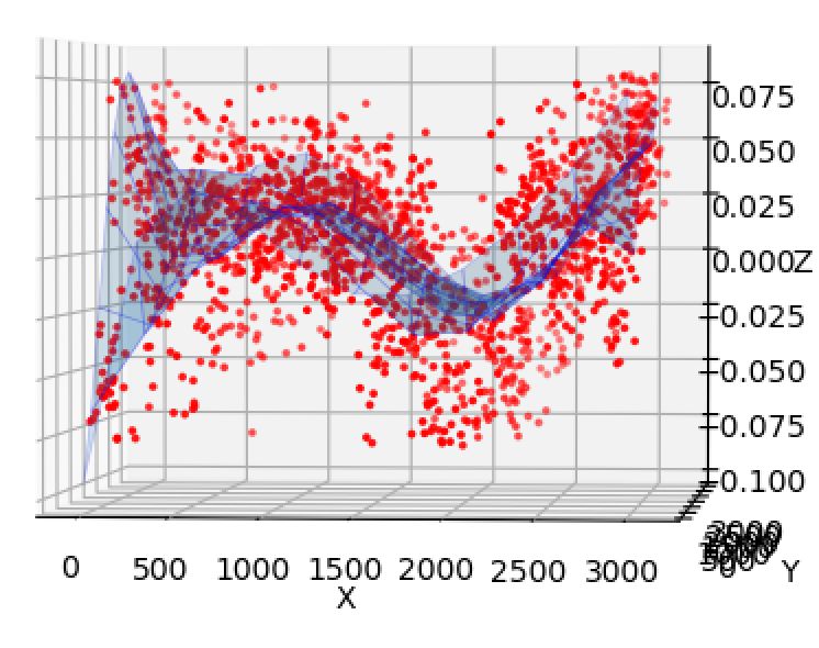
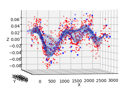
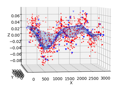
Spatial residuals and fits to r-band obsevation of ZTF field 592 taken on 2020-02-24 calibrated to PS1 for CCD-6 quadrant 1. The grid represents the surface fit usung multiquadric radial basis function to the data with smoothing=0.5.
In the plots above we show how the residuals are modelled with a multiquadric radial basis function. Compared to the same fits on this data we see the surface is represented much better using this fitting. However, unlike the other fits it is difficult to weight the data points based on their expected uncertainty. Thus it necessary to limit the data to points with uncertainties smaller than the amplitude of the structure.
Which fit is the right?
In order to find the best fit to the surface data it is necessary to consider which model best fits the data with over fitting it. Higher order fits automatically reduce the residuals of a fit but do not neceassarily better represent the underlying distrbution. In very high order fits ringing occurs where the fit is poorly constrained.One way of determining the best model is to use Akaike information criterion (AIC). This quantity does not determine which model is correct, but which is best among a set. To choose the correct model we simply fit a sequence of model and select the model with the lowest AIC. This method also provides a means of determining the probability that other models with similar AIC values are better than that with the lowest value.
Another method is to use the Bayesian information criterion (BIC). In comparison to the AIC this more strongly penalizes models with more parameters.
For the polynomial fits we use AIC values to determine the best model. However, for smoothed radial basis function fits it is difficult to determine accurate AIC values since the method account for unsmoothed data.
In the plots above we show the fits for multiquadric radial basis fits for different smoothing values. Here we see that there are quite different fits depending on smoothing. To estimate which among these is best we need to use a different method.
Validation of RBF fits
Since it is difficult to determine an appropriate AIC value for smoothed radial basis function fits we will use an alternate method. Rather than using all the data in the fitting process we randomly remove 10% of the data and use that data to validate the fit.

In the above plots we can show an RBF fit. Here we can judge the accuracy of this fit relative to other types of fits based on the scatter in validation dataset. In principal we expect that the most reasonable fit will be one where the residual scatter in the fit data is similar to the validation data. A more robust validation would be to perform the fit multiple times, leaving out different sets of data each time, then comparing the results. However, this is currently not practicle due to the amount of time perform multiple fits on every frame takes.
Discussion
In this analysis we discovered that many of the individual ZTF frames exhibit strong spatial structure in the residuals due to variations in transparancy. To correct these we fit each frame with multiple polynomial surface fits. In cases where there are limited numbers of calibrator sources we limit the degree of the polynomial since the fits become unstable. This means that such structure in sparse field may be poorly modelled.We determine the best fitting model based on AIC criteria. However, when the best fit is a high order polynomial we additionally perform RBF fits with multiple levels of smoothing. We then choose the best fit among these cases based on the scatter in a validation set.