| Topics |
|---|
| Spatial structure variations over time |
| Spatial structure variations with colour |
| Accurate spatial structure variations in g-r |
| Spatial structure variations with g-r |
| Discussion. |
Variation in Spatial Structures Over Time
Besides the presence of a varying gain with sky level it is worth considering how the spatial structure of the resiudals might have changed over ZTF-I.
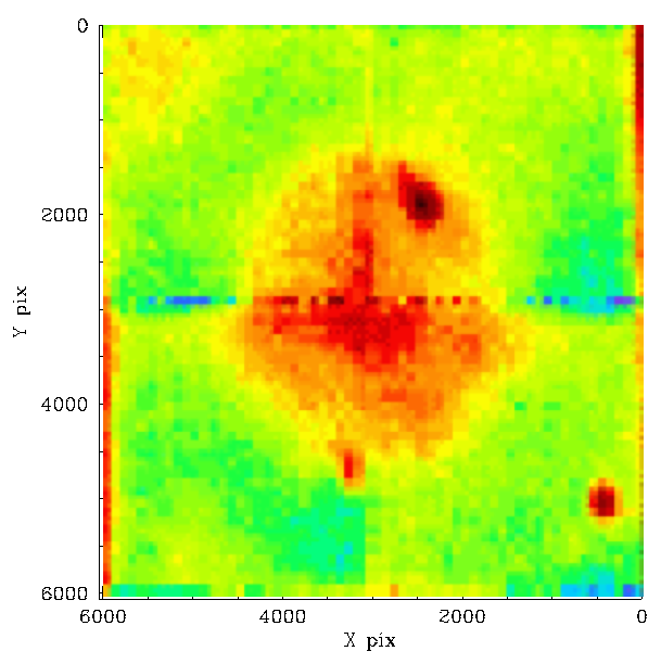
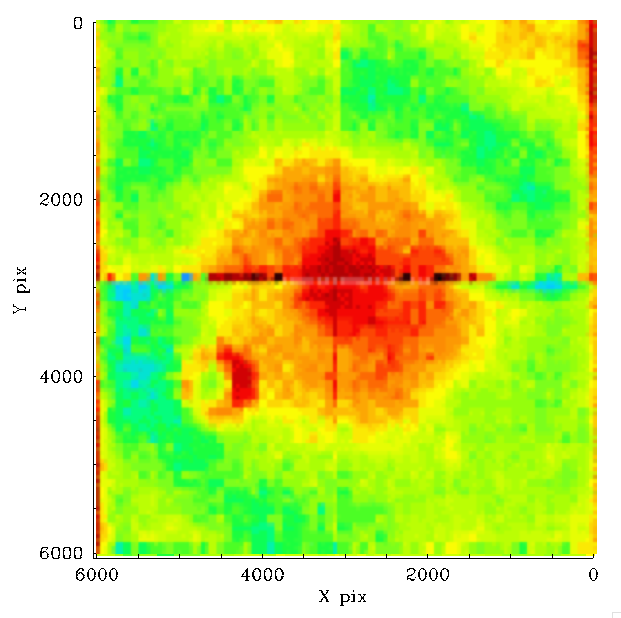
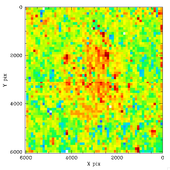
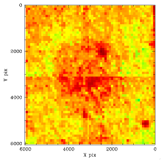
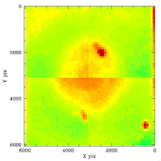
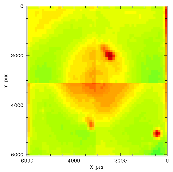
Spatial structure of g-band calibration residuals (PS1 - ZTF) for ZTF CCD 6.
In the plot above we show the spatial structure that was determined earlier based on the combination of median magnitudes from 30 ZTF fields. With our Zubercalibration we are able to determine the spatial structure by combining results from a single night such that any variations during that time cane be seen.
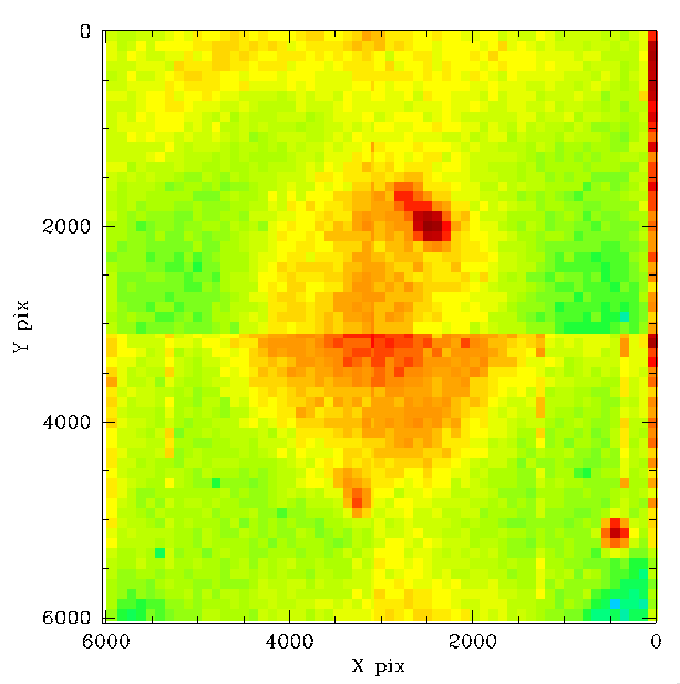
In the above plots we show the g-band spatial structure derived from six nights spanning most of the observation range of ZTF-I. Here we do not see many obvious changes in the spatial structure, and since the scaling is the same in each plot, we can say that the ampitude of the structure does not vary by much either (as expected based on the flat fields above). However, in a number of the individual nights we see vertical lines in some quadrants that were not present in the combine field analysis. It is likely that these effects are real and were smoothed out in the combined analysis. In the above plot each pixel is generally the average or two to three hundred sources with mag g_inst < -7 (g ~ 19).
In order to better quantify how the structure varies between nights we bin the values from each of the pixels. As we can see the overall distribution of pixel values does not vary much across the six nights. In general there are fewer values near zero than the average of the six nights and more tail values since the individual night data is noisier than the average. This is particularly clear for 2020-02-24 and 2020-03-06.
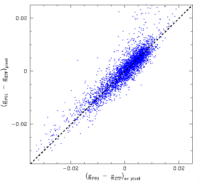
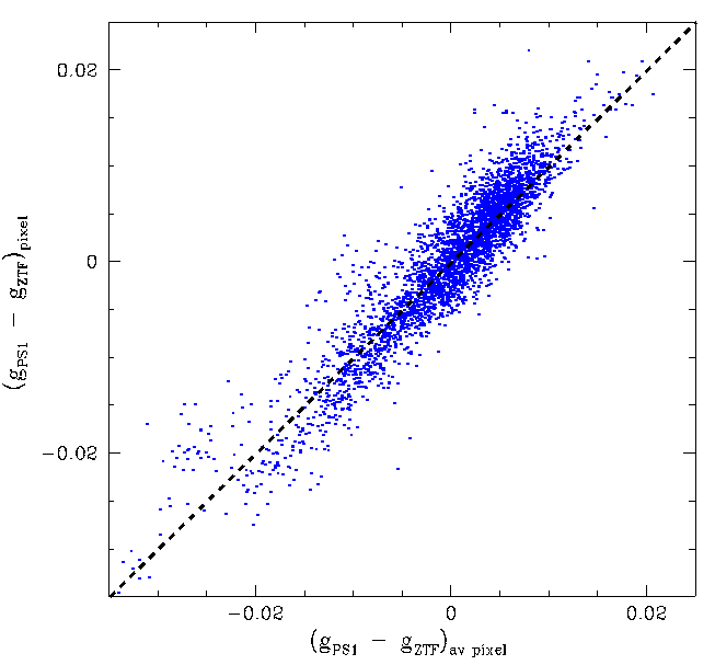
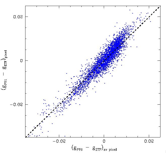
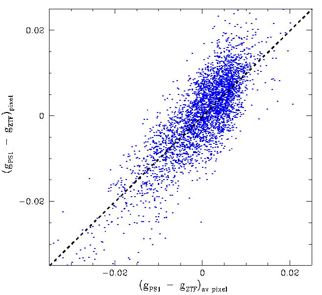
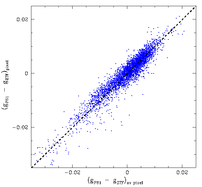
To better quantify the variation in residuals at the locations of individual pixels in the plot above we compare the values from each night with the average of the six night for the 900 pixel bins. Here we see that the images generally obey the expected linear trend, with scatter that is generally < 0.005 mags. The data from 2020-03-06 is notably noisier as expected from the image above. In this case and others there is some evidence of deviations from the linear trend, suggesting that there may be slight changes in the structure.
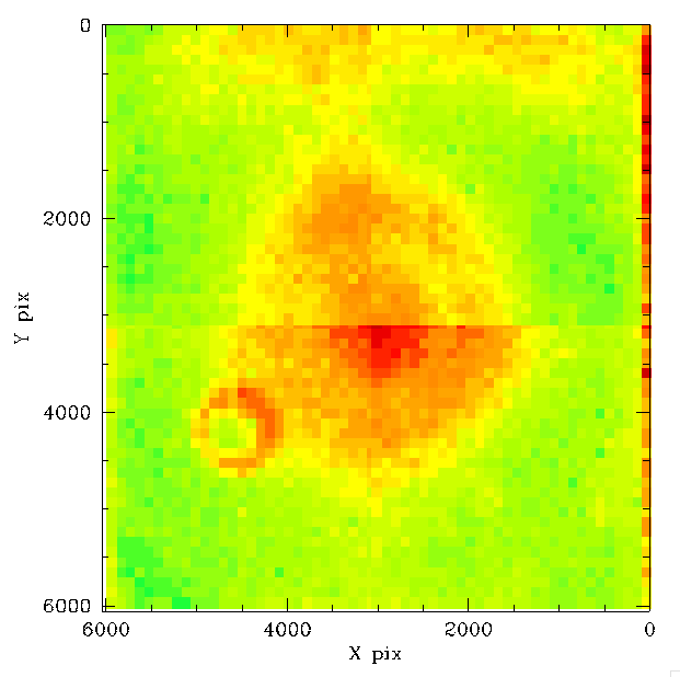
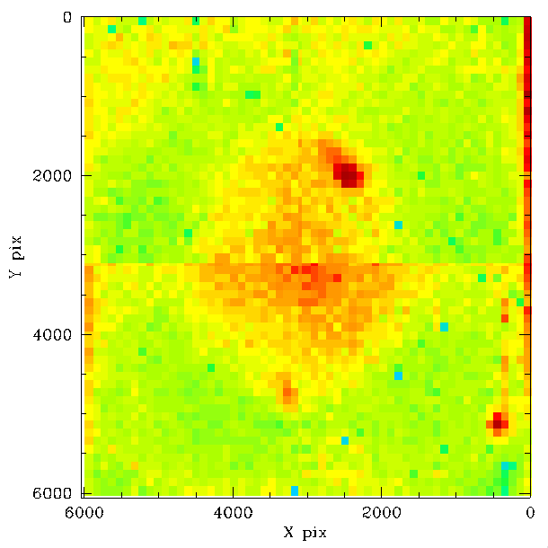
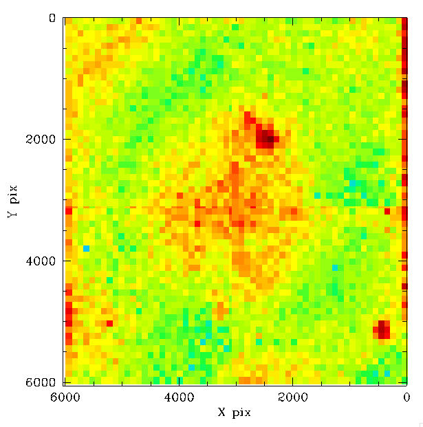
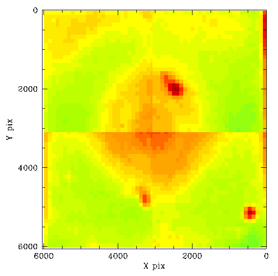
As a comparison to CCD-6, which varies significantly overtime, we show the structure for CCD-7 above. As with CCD-6 we see that the general strucure is consistent with the prior analysis. Note the colour scaling of these two images is not exectly the same.
Spatial structure variation with source colour
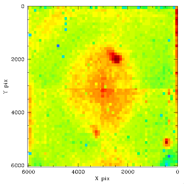
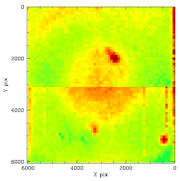
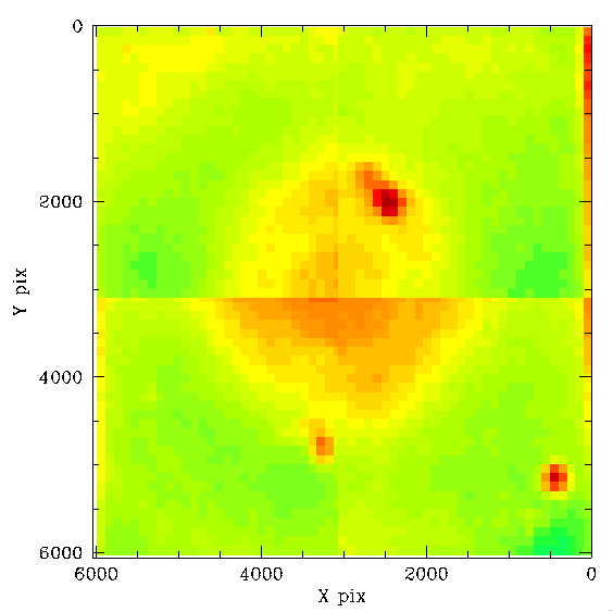
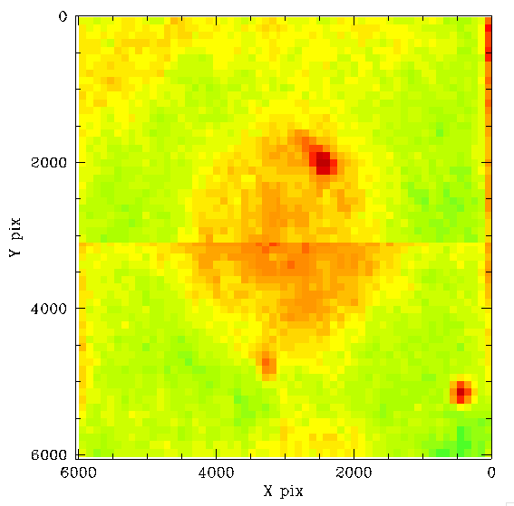
To improve the signal-to-noise ratio of the above individal image we average the pixel values from six nights of data.
The plot above shows the combined structure that is consistent with earlier results. Each pixel bin includes ~1400 stars. Note: the colour scaling is not exactly the same.
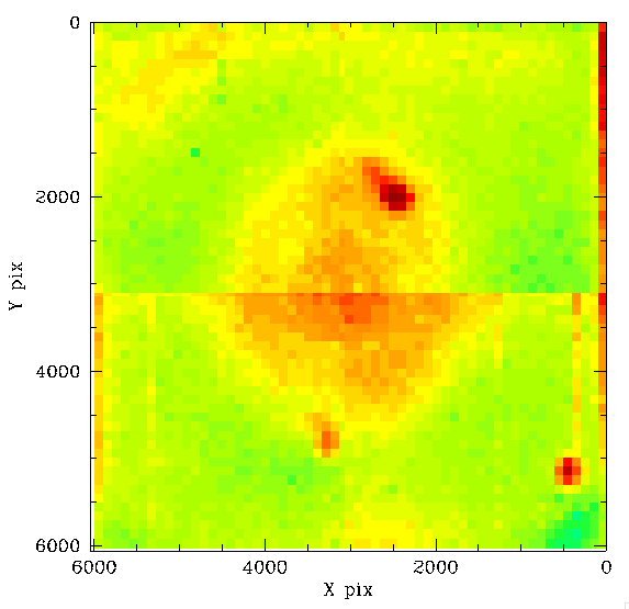
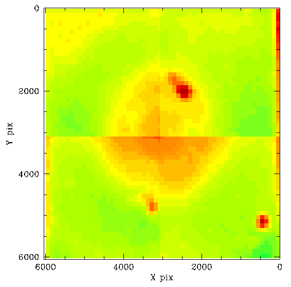
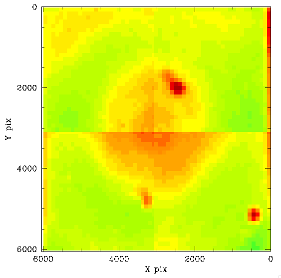
To determine whether the spatial residuals are dependent on the colour of the source we divide the sources by g-r colour and average over the six nights of data.
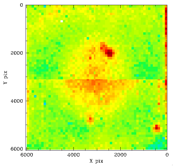
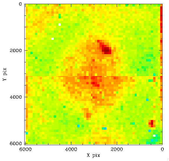
In the plot above we see that there is indeed some variation in the scale of the spatial structure with source colour. In particular, the structure is much stronger for the redder sources. This relates well to the colour dependence seen in the flats. Note, the red sources will tend to be fainter than the blue ones on average, so the result is expected noisier. However, each pixel in the red sources image include ~350 sources, while each blue pixel includes ~200 sources.
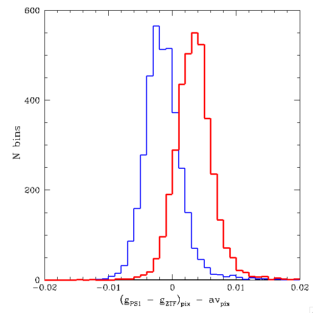
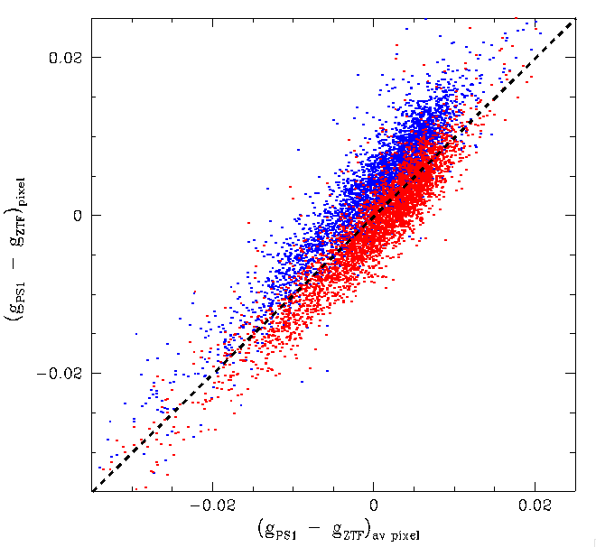
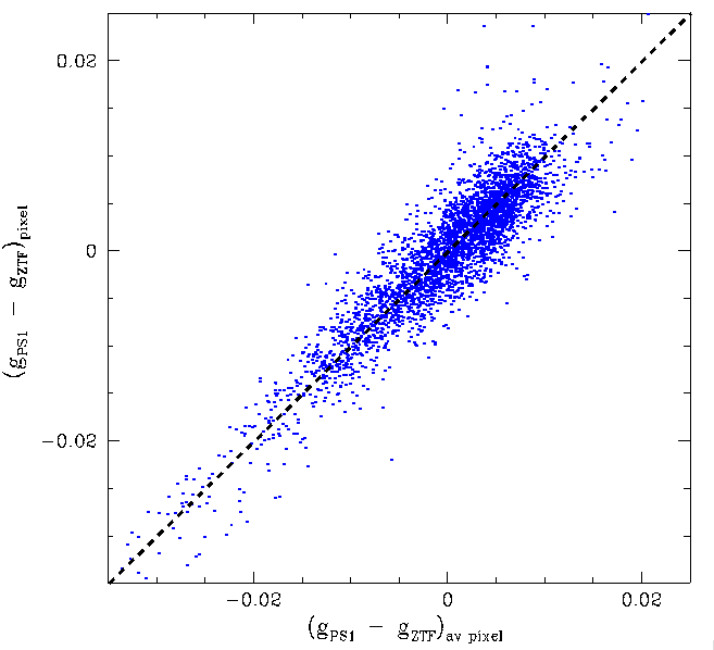
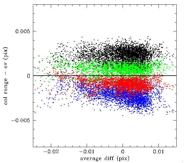
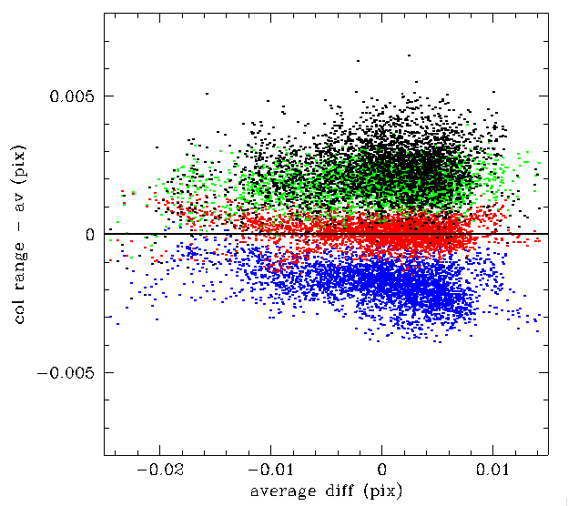
To better quantify the difference between the blue and red sources we determine the binned pixel-wise difference between residuals based on blues sources (g-r < 0.4) and the average of all stars, and residuals based on reds stars (g-r > 0.8) and the average. In the plots above we clearly see that the scale of the photometric residuals varies systematically between blue and red sources.
The right plot above shows that, no only are the residual larger for red sources than blue, but the sources are systematically slightly offset from the average for every value. Thus the correction used to correct for the spatial residuals is colour dependent. The average corrections currently used can be wrong by ~5 millimags depending on the source colour.
High S/N analysis of ZTF spatio-chromatic photometric variations
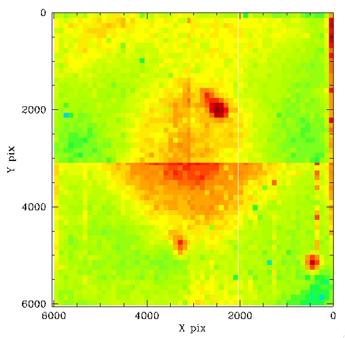
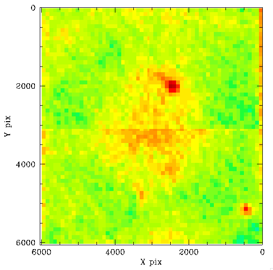
In order to investigate how the residual spatial structure of ZTF data calibrated to PS1 varies with colour, we recalibrated 725 nights of ZTF-I g-band data for CCD6 using our Zubercal process (Further details will be presented elsewhere).For each night we bin the photometric residuals from each calibrated quadrant image into 30x30 bins. We then determine the average structure of all nights as with the data above. The combined data consists of ~200,000 calibrator measurements per pixel.
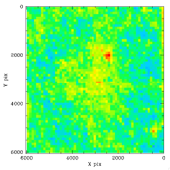
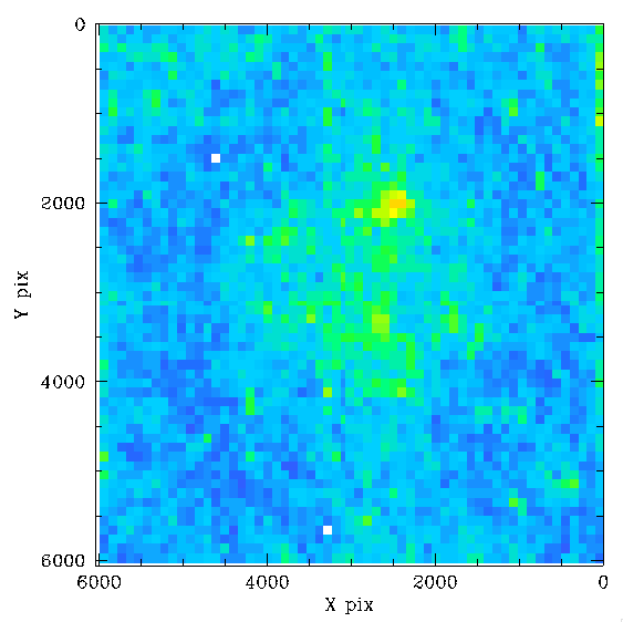
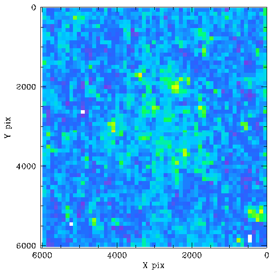
We then subdivide the measurement sources in each pixel by their g-r colours to determine how the observed spatial structure varies with source colour (due to varying CCD thickness that produces a spatial colour dependence.
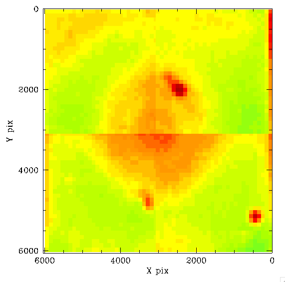
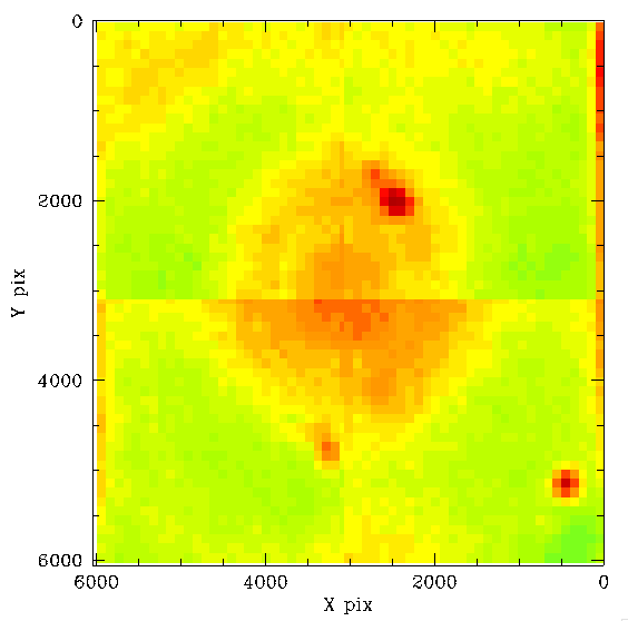
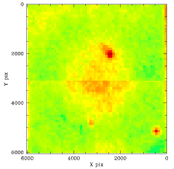
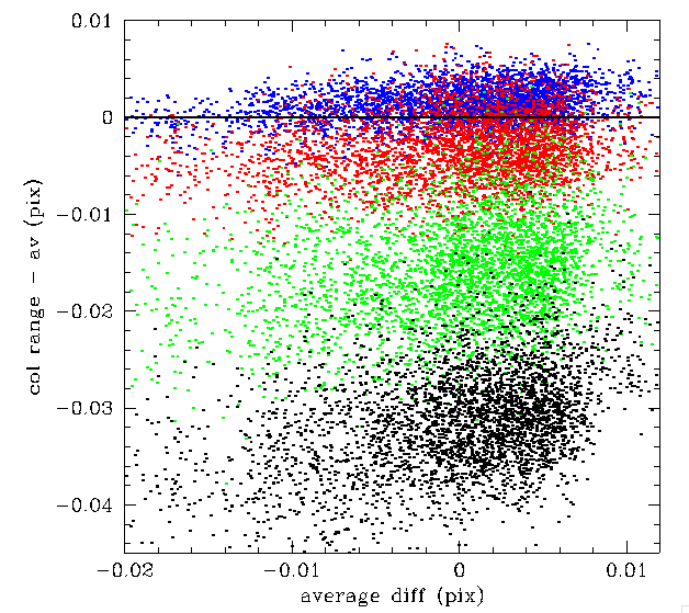
In the plots above we show how the residual spatial structure changes for sources with varying g - r colours (range 0 to 2.0). Clearly the spatial structure we see is strongly dependent on source colour. In the first and last bins there are limited numbers of calibrators so the plots are noisy. Taking the values from each spatial and colour bin we look at the variation relative to the average structure from all sources.
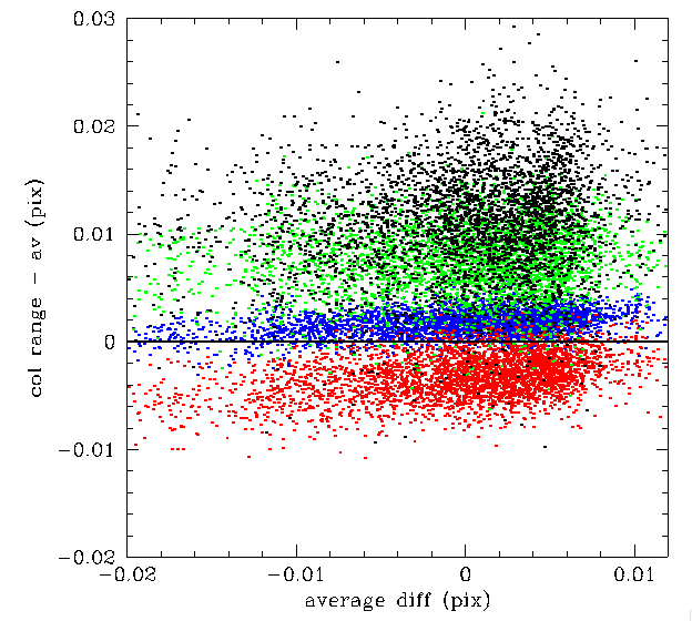
In the above plot we see that the main effect of colour is an offset from the average residual spatial structure within a pixel. The behaviour is evidently somewhat complicated since the offset relative to the average does not purely increase or decrease with source colour.
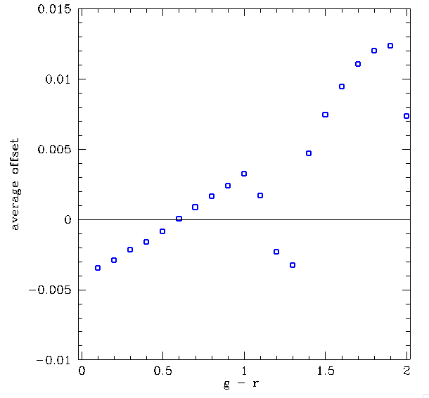
We determine the offset from the average structure for each g-r colour bin averaged over all 900 pixels of the images above. The residuals were rebinned to provide additional g-r values. In the plot above we show how this residual varies from the average for varying source colour. The plot is clearly somewhat complicated since sources in the g-r range of 1.0 to 1.4 break away from the general trend. This is likely caused by the degeneracy of late star types with PS1 g-r colours previously found.
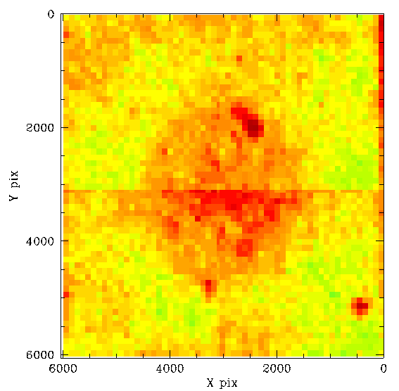
Spatial residual variations with PS1 r - i colour
Here we repeat the analysis above, but divide them by their r-i colours since these values do not suffer the same degenerate problems as g-r colours.

In the plot above, as expected, we see similar residual structure as when the data was divided using sources g-r colours (above). Here the final two plots are noisy due to small numbers of red calibrators.
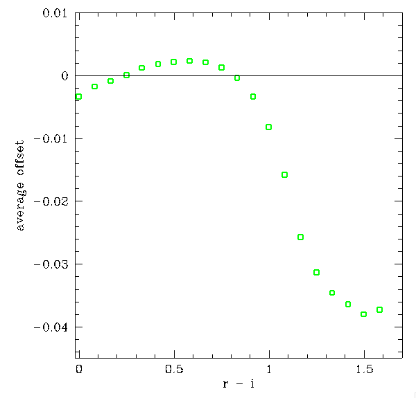
In comparison to the variations with source g-r, the plot above is well behaved since r-i data does not suffer the stellar colour degeneracy. However, the scale of the difference is much larger for very red sources. So inaccurate values of r-i could lead to large errors in a correction for source colour. Additionally it is not completely clear that the variation with source colour is purely an offset. Indeed, the locations of large dust spots appear to have a different dependence and there is some structure in the variations from the average.
More work is require to determine whether there is any temporal dependence in the spatial structure.
Discussion
After using Zubercal to remove the gain (brightness) variation we see very slight changes in the amplitude of the spatial residuals. These changes are not easily explained by other non-spatial errors in the calibration.
By combining the residuals from multiple nights, and separating sources by colour, we see that the spatial residual structure varies very strongly between blue and red sources. Current corrections to ZTF photometry for spatial structure can be wrong by ~5 millimags depending on the source colour.
By fitting 725 nights on ZTF g-band for ZTF we were able to determine the PS1 g-r and r-i dependence of the ZTF spatial structure caused by varying CCD thickness. This can thus be applied to determine more accurate absolute magnitudes of sources.
More work is require to determine whether there is any temporal dependence in the spatial structure.