| Topics |
|---|
| Improving ZTF data quality. |
| Changes in ZP baseline over time. |
| Colour and RMS cuts |
| Combined cuts |
| Extinction Variations in ZTF exposures |
| Discussion |
Improving ZTF data quality
In 2019 we undertook a small analysis in order to improve the average data quality of the first ZTF DR1. This analysis was limited to the analysis of 60 ZTF fields. The cuts used consisted of a single ZP threshold per quadrant adjusted for airmass. Cuts were also applied based on the ZP RMS and the number of PS1 calibrator stars matched in the calibration process.More recent analysis has shown us that ZP are far from stable over time . Thus, it is necessary to understand both instrumental and weather based changes in selecting good data.
Changes in ZP baseline over time.
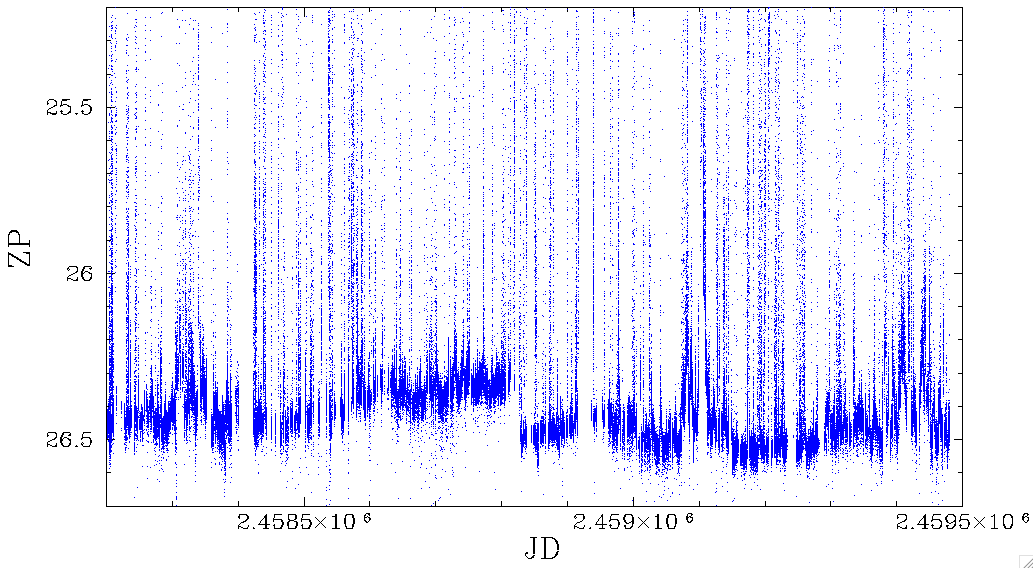
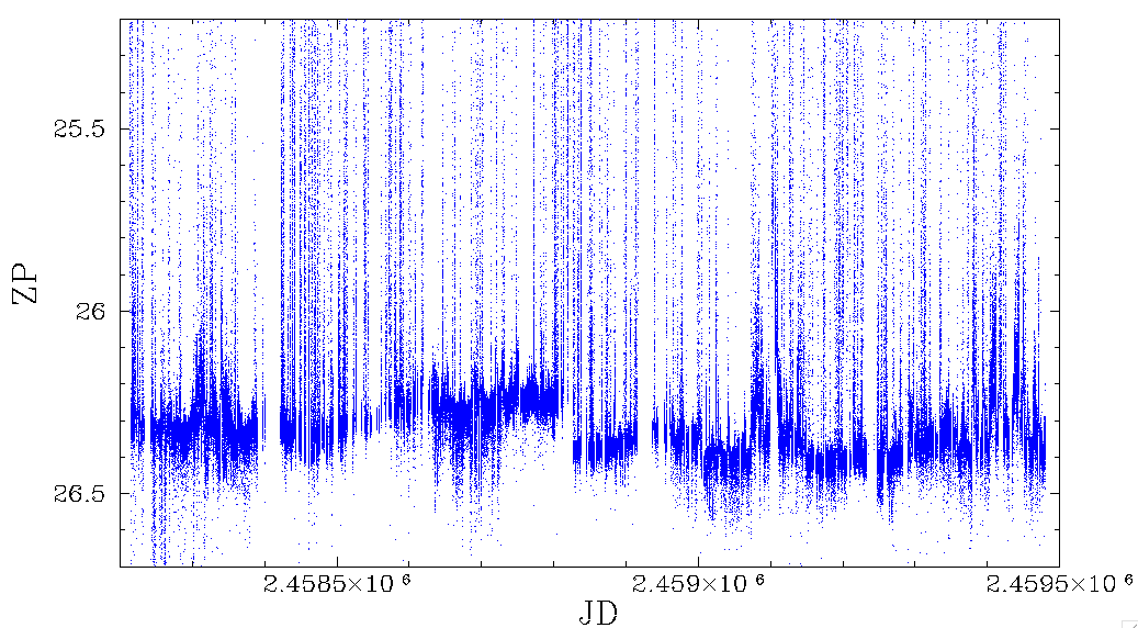
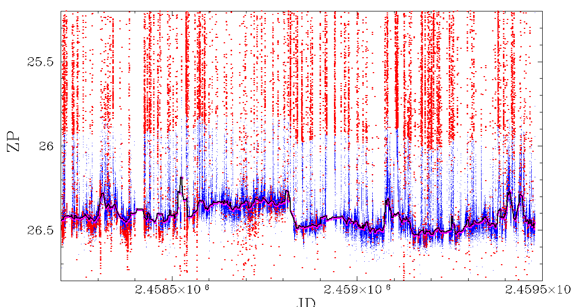
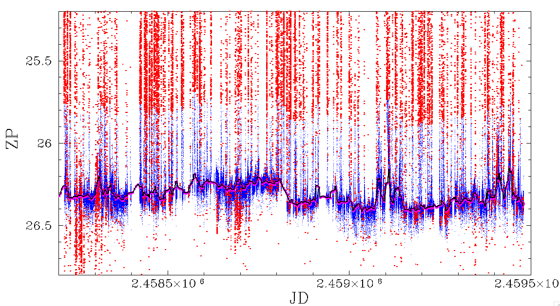
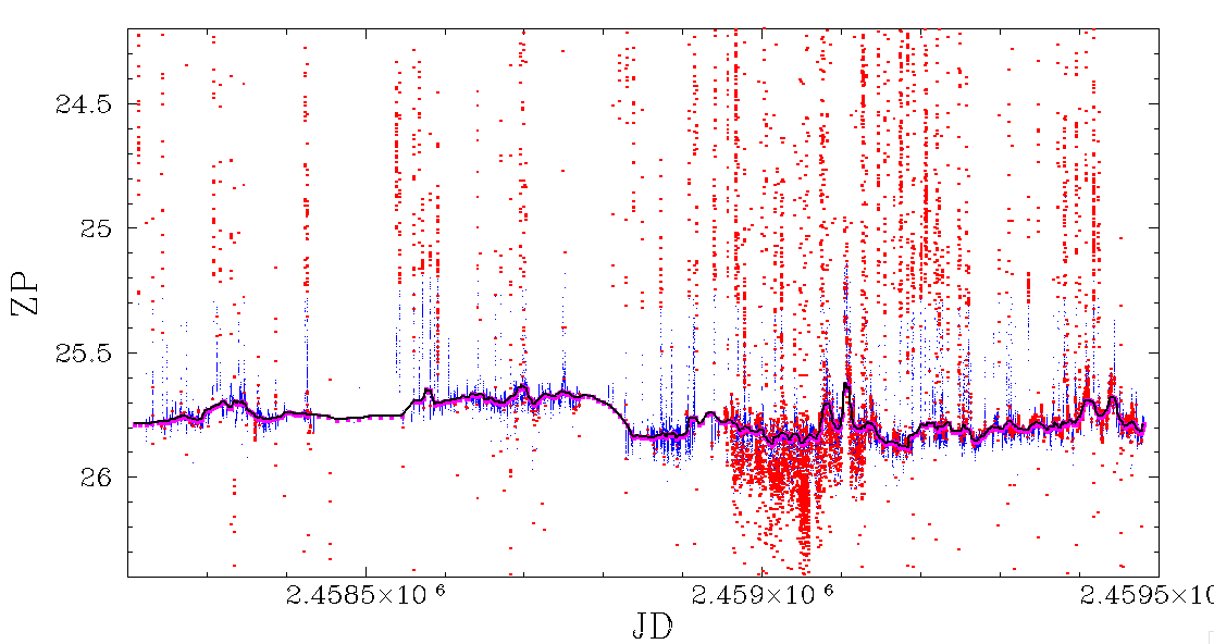
The first step is to see how the ZTF calibration zero points change over time.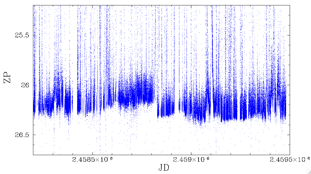
In the plots above we show how the zero point varies during the ZTF-I and ZTF-II, for three quadrants taken in the three different filters. We clearly see significant variation where the bulk of data follows a trend that is seen in all filters. Above the main trend line point deviate to lower ZPs due to the presence of clouds that reduce the depth of the images. The amount of extinction on a cloudy night typically varies from one image to the next. This is difficult to predict since the observation sequence generally moves from one field to the next. We have verified that the underlying trend is very similar between all quadrants.
In the case of the i-band observations we see a significant deviation in the baseline. this due to longer observations being taken during two periods of time. Clearly quality cuts can not be applied to i-band data without considering this.
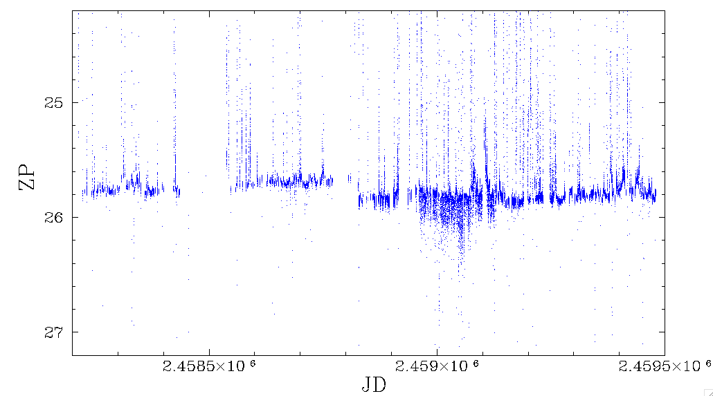
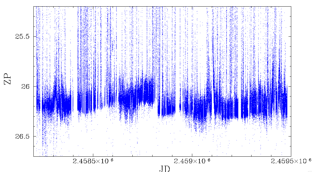
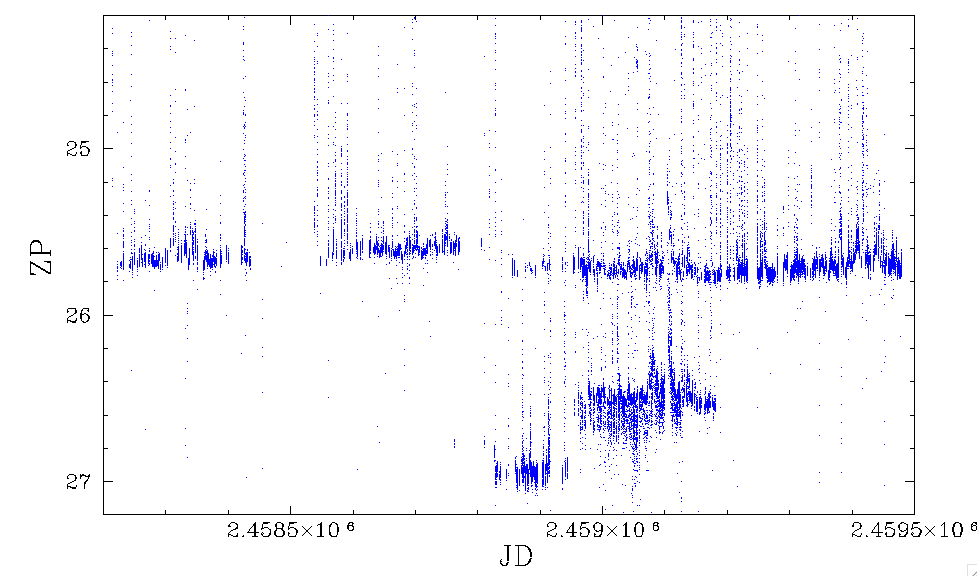
In the plots above we correct the ZPs for variations in exposure times as well as variations in airmass between observations. Here we see the baseline of observation ZP is much narrower yet still varies significantly.
When we consider the band of maximum ZPs we see that there are short and long trends. On short timescales it is possible that long term weather can effect the baseline. On long timescales the trends must be due to instrumental variations. These include the build up of dust on the instrument as well as variations in electronics.
In order to quantify the underlying trend we determine the median for each date. The nightly medians are biased by the cloudy observations, so we determine the median value of the nightly median and remove points outside a window based on the underlying variation. We then do a running weighted average of the remain values.
Colour and RMS cuts
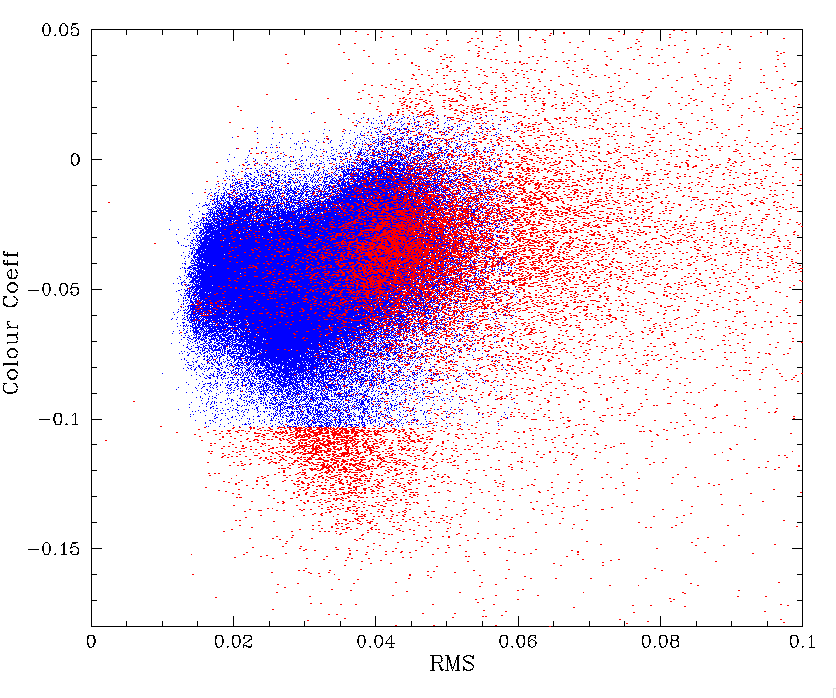
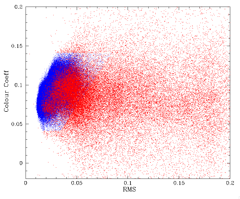
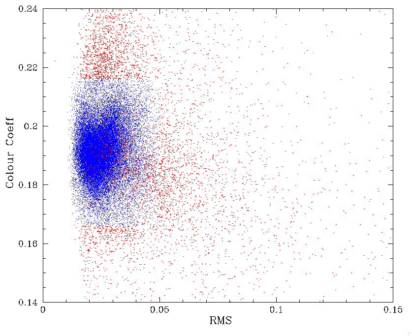
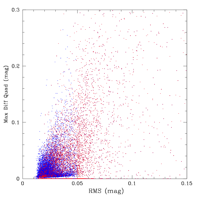
In addition to zero point values we can select bad data based on the RMS of the ZPs as well as the colour coefficents in the calibration fits.
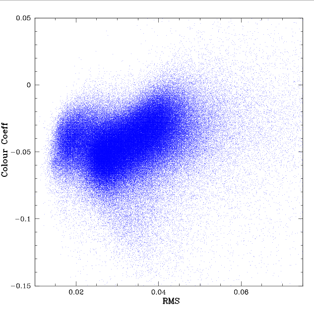
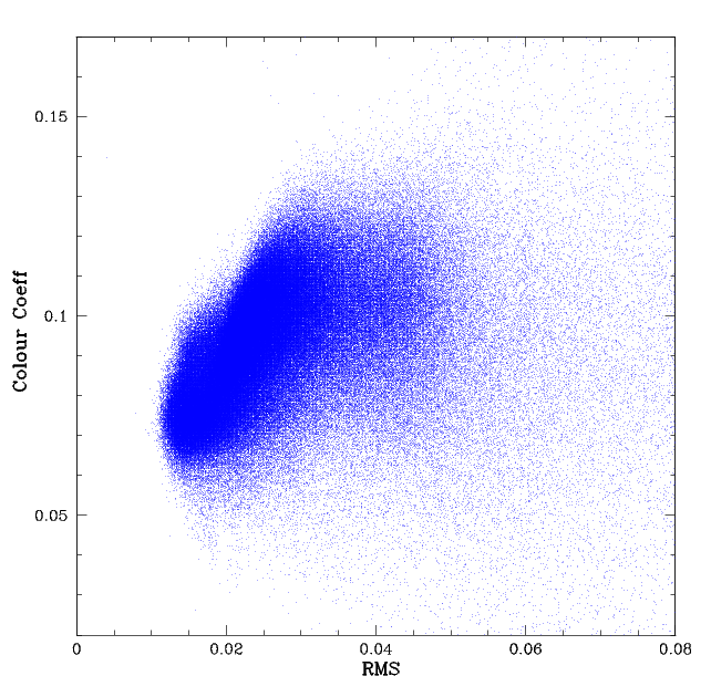
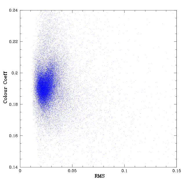
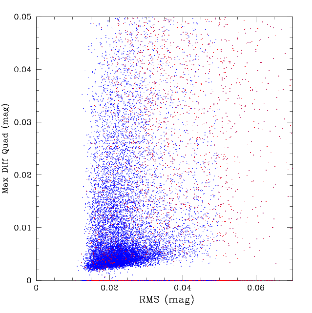
In the plots above we show the ZTF colour coeffs and ZP rms values for all observations taken within three quadrants for the three ZTF filters. Here we see that there are observations with RMS outliers many times the typical values. In many cases the outiers are due to varying extinction within a frame. We also see that many of the RMS outliers are also outliers in their colour coefficients.
We apply RMS cuts of 0.06 in g-band and 0.05 in i-band. For r-band we see that the RMS increases with colour coeff. So we apply an RMS cut that varies with colour coefficient. We also apply cuts in colour coefficients. However, we know that the colour coefficients vary strongly with camera quadrant and filter. So we set a window that varies with the median colour coefficient within a given quadrant and filter combination.
Combined cuts
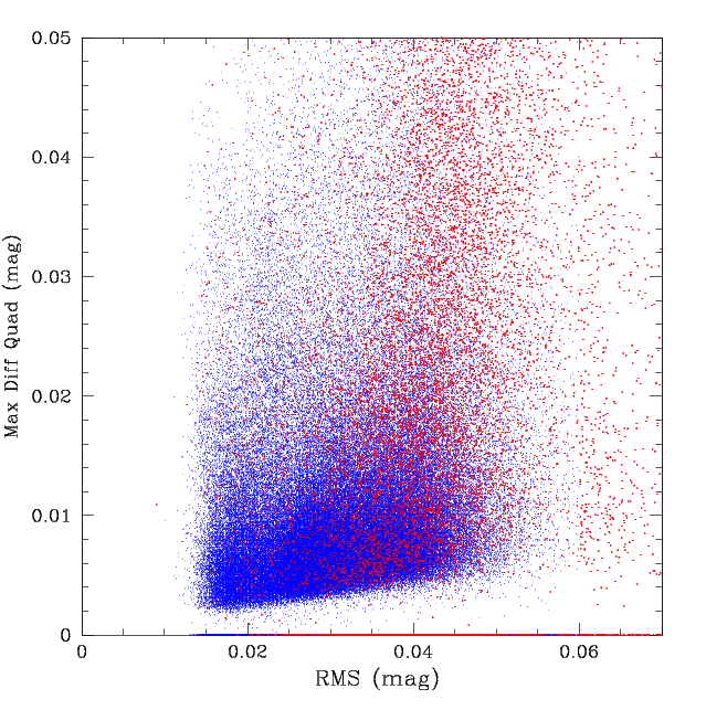
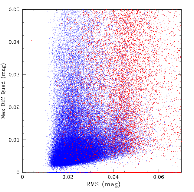
In the plots above we show the time distribution of bad data based on selections based on variation from the running baseline ZP as well as cuts based on RMS and colour coefficients. For consistency with our prior cuts, we generally remove observations that are 0.5 mags above or 0.3 magnitudes below the expected zero extinction level for a night. As a second optional cut we remove frames 0.3 mags above the expected value.
In the plots above we show the distribution after including the cuts on ZP, ZP RMS and colour coefficients.
| Frame selection stats | |||
|---|---|---|---|
| Total | Cut (fraction) | Cut2 | |
| 16883983 | 2113079 (0.125) | 2474661 (0.146) | |
| 25193038 | 2661944 (0.106) | 3138473 (0.125) | |
| 3081478 | 357561 (0.116) | 399801 (0.130) | |
In the table above we give the number of frames cut by our selections.
Extinction Variations in ZTF exposures
As we have previously discussed, the regular ZTF calibration involves determining a single zero point for each frame. However, we know that this solution is far from accurate in the presence of clouds. In fact, many images have very siginificant spatial structure in the amount of cloud-based absorption. However, although many individual images have small scale structure that is corrected with Zubercal, it is worth considering if the data affected by clouds should even be included in data releases.To determine the amount of extinction we first correct the ZPs for time-based trend above. The variation from the nightly model values for each filter should mostly be due to atmospheric extinction (some field-based variation may also be present). Thus if we look at the ZP variations for all 64 quadrants within any given exposure we should be able to see how uniform the extinction is.
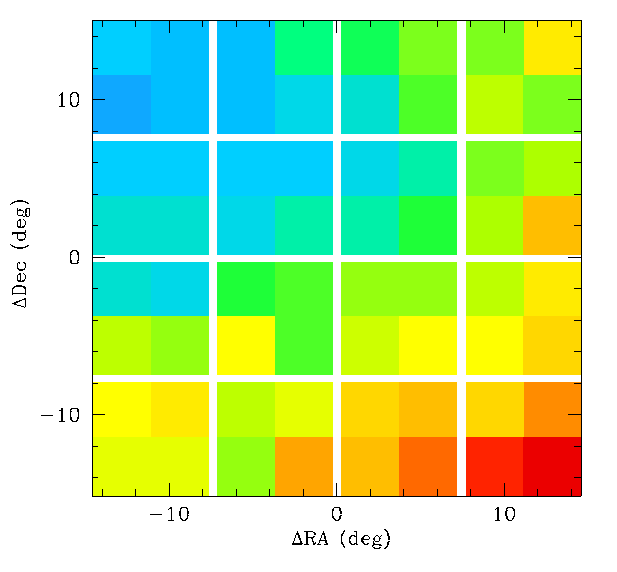
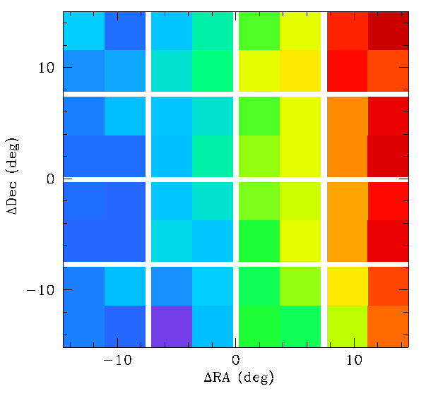
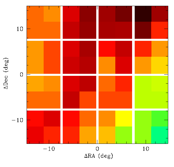
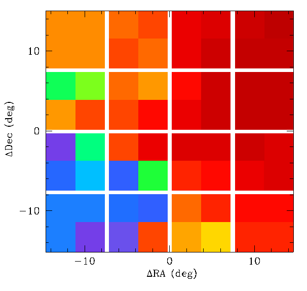
In the plots above we show the variation in exinction across the 64 quadrants of the camera for four different exposures. Here we see that the individual observations can have widely varying extinction across the ZTF FoV. As the regular calibration has a single ZP per quadrant, any gradient in extinction is not corrected. Additionally, in becomes clear that, although a frame may exhibit very little extinction (and thus be considered good in the cuts above) it can still have a significant gradient that would suggest it should be excluded from a selection of photometric data. Since the value of ZP RMS for a frame is dependent on the number of calibrator stars, we cannot simply use high values to remove such frames.
In order to improve the photometric quality beyond the new cuts applied above, we use the ZP values from the 64 quadrants in each observation to determine the presence of spatial varying extinction. For every g,r, and i-band observation we fit surfaces to the ZP values after clipping extreme outliers.
The surface fits range from a constant to a fourth order polynomial surface (there are insuffient points for higher order fits). We then use the AIC criteria to select the best fit from five fits.
| ZP Fit Stats | ||||||
|---|---|---|---|---|---|---|
| None | Constant obs (fraction) | poly_1 | poly_2 | poly_3 | poly_4 | |
| g | 0 | 91451 (0.35) | 133303 (0.50) | 22374 (0.08) | 9913 (0.04) | 7578 (0.03) |
| r | 0 | 146589 (0.37) | 160583 (0.41) | 41129 (0.10) | 23294 (0.06) | 21390 (0.05) |
| i | 0 | 28519 (0.59) | 10723 (0.22) | 3562 (0.07) | 2740 (0.06) | 2455 (0.05) |
In the table above we give the number of exposures in each filter with the best fit of each type along with the fraction of the total number of exposures. The "None" case specify to just use the nightly zero-extinction value. We see that a constant extinction across the full focal plane is always better than no fit. i.e. there is always a slight offset. This may be due to the slight field offsets noted earlier.
Interestingly, we see that a constant exinction is only the most common in i-band. In other filters, a first order polynomial is the best fit in most cases. Indeed 50% of g-band observation exhibit evidence for a gradient. Thus, most g and r-band ZTF exposures have extinction gradients at some level. Most exposures do not appear to have complex structure since the fraction of high order fits is low. Nevertheless, considering all the higher order fits, a large fraction of the exposures do appear to have more structure than a simple smooth gradient.
In order to determine the amplitude of the varying atmospheric absorption across each quadrant image we calculate the values of extinction at the corners of each quadrant based on the fits. From the four values we find the maximum variation in extinction. In cases where the best fit is a constant, there are no variations. We bin the results so that we can see the fraction of frames with a given level of spatial extinction variation (that is not accounted for in the regular ZTF calibration process).
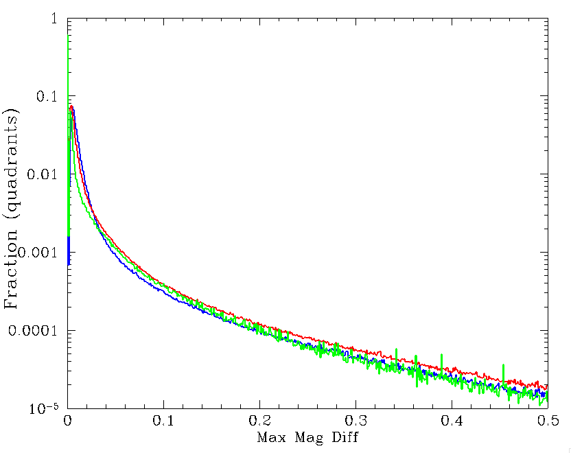
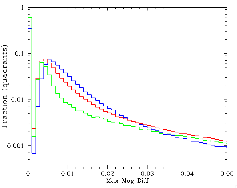
Histograms of the predicted maximum variation in absortion across each
ZTF quadrant image. The right plot is a zoom of the left.
The blue, red and green lines denoted the g, r and
i-band values, respectively.
In the plots above we see that large spatial variations in extinction are uncommon. However, there are images with extinction variations greater than 0.1 mags across the frame. However, the right plot above shows that there are many frames with greater than 0.01 mag variation. These frames cannot be accurately calibrated with a calibration single fit and are expected to give rise to significant photometric noise. Note, the spike at zero occurs where the best fit is a constant. This feature is somewhat artificial since it only means the variations within quadrants were too small to determine with fits on large spatial scales (the full ZTF FoV).
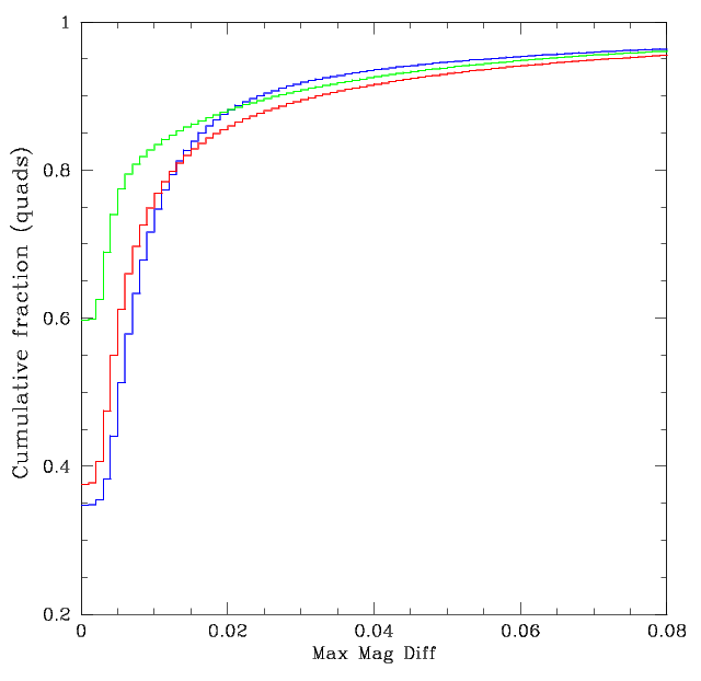
In the plot above we show the cumulative fraction of quadrants against the predicted maximum in extinction across a quadrant. Here we see that 95% of quadrants are expected to exhibit extinction variations of less than 0.08 mags. However, these fits have too few points to detect the fine scale structure seen within quadrants using Zubercal.
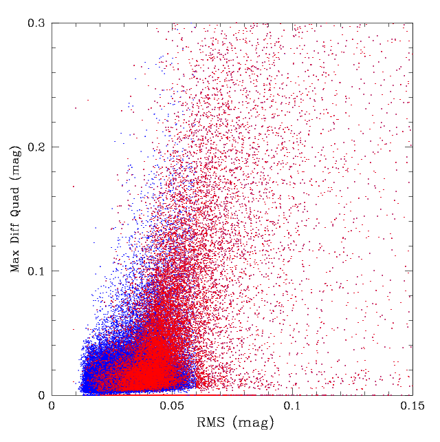
In the plots above we show how the maximum variations in expected quadrant ZPs, due to extinction, varies with the ZP RMS from the standard ZTF calibration. As expected larger ZP RMS is correlated with larger variations in the ZP within a quadrant. We see that frames with the largest variations in ZP within a quadrant are removed by our RMS selections. However, there are clearly still frames with significant gradients that have not been removed. We therefore add a cut on the maximum values for each filter. The combined cuts remove ~13% of observations in each band.
For photometric data we generally require variations of less than 0.01 mags. This occurs in more than 70% of frames. However, there is a very large variation in the number of photometric frames between bands. This is likely due to the fact that atmospheric absorption can be wavelength dependent. In particular, Aerosols and Rayleigh scattering produce far more extinction at blue wavelengths than red. However, significant variations in these components on sub-degree scales appears much less likely than clouds (which are often noted as being gray absorbers). Nevertheless, there is strong evidence that the exinction observed within ZTF filters is colour dependent in some cases. A stricter set of cuts was also made that removes ~19% of observations.
Discussion:
We have developed a new set of cuts to replace those original designed for ZTF DR1. Unlike the original cuts the new ones take into account the time dependent variation of the baseline ZP for each quadrant and filter. The number of observations flagged has been set to be very similar to the current cuts. However, an additional more stringent set of cuts, which removes few percent more observations, can also be applied if higher quality is desired. Unlike the original set of ZTF DR1 cuts, we also cut some observations based on outlier colour coefficients. However, we do not flag observations based on the number of calibration stars.In our selection we apply corrections for exposure time and airmass. The airmass corrections are 0.184, 0.11 and 0.07 mag/airmass in g,r and i-bands respectively. This varies from the 0.2 and 0.15 mags previously used for g and r since the prior analysis did not account for the time variation (which gives rise to a much broad envelope of ZP values). Our Zubercal ZP analysis for CCD1 also gave rise to slightly different values of 0.178 and 0.088 for g and r. In r-band there is almost certainly some variation between CCDs due to the coating on the central CCDs. So some variation is expected.
In order to better understand whether additional selections are required to remove poor quality observations, that might be missed by simple cuts of ZP, ZP RMS and colour coefficient, we have carried out ZP surface fits for all ZTF frames. This enables us to gauge the extent of spatial variations in extinction within ZTF images in a way the selections based on the individual quadrant ZP values do not probe.
For ZTF observations in g and r-bands we find that most images have significant structure. For i-band most images have constant level of extinction. In all bands, around 20% of images exhibit more complex structure.
We use surface fits to ZP variations from across the ZTF focal plane to determine the level of extinction variations within individual quadrant images. We find ~20-30% exhibit internal variations of > 0.01 mags depending on the ZTF filter used. These images must be considered when selecting the best quality data.