| Topics |
|---|
| Determination of the Extinction ZP. |
| ZP variation with field and other params. |
| Time dependence. |
| Trends with the number of catalog sources. |
| Field offsets. |
| Checking model dependencies. |
| Other noteworthy trends. |
| Conclusions. |
Motivation
In part 1 we started exploring the Uber calibration of ZTF photometry. We discovered that this process requires understanding of both atmospheric extinction as well as variations in the throughput of the telescope.Determination of the Extinction Zero Point
One of the main problems in calibrating ZTF photometry in the presence of atmospheric absorption is that this it is likely to vary between one field an the next in an uncertain way. In most cases this is unlikely to be a smooth transition but rather a step function. Thus, it is not possible to fit a smooth function to determine the amount of absorption as a function of time. However, if one is able to determine the point where there is maximum throughput for a field, it may be possible to estimate of the amount of extinction in each observation. Determination of this estimate is complicated by presence of concurent variations in the instrument itself.As an initial estimate of the zero extinction for each field we found the the maximum ZP value in each field after removing spurious values based on the DR1 cuts, removing observations with exposures longer than 30 seconds, and correcting the image zero points for airmass (which is the main reason for ZP variations). The expectation was that these values would not be as accurate as desired (< 0.01 mags) since there is likely to be a very slight amount of extinction even during the best observing conditions.
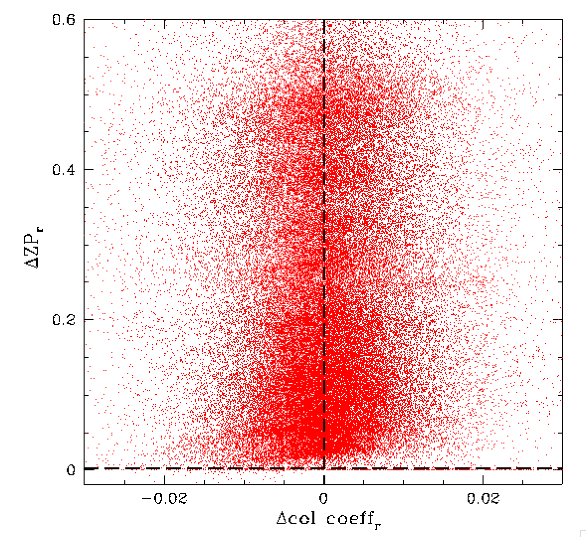
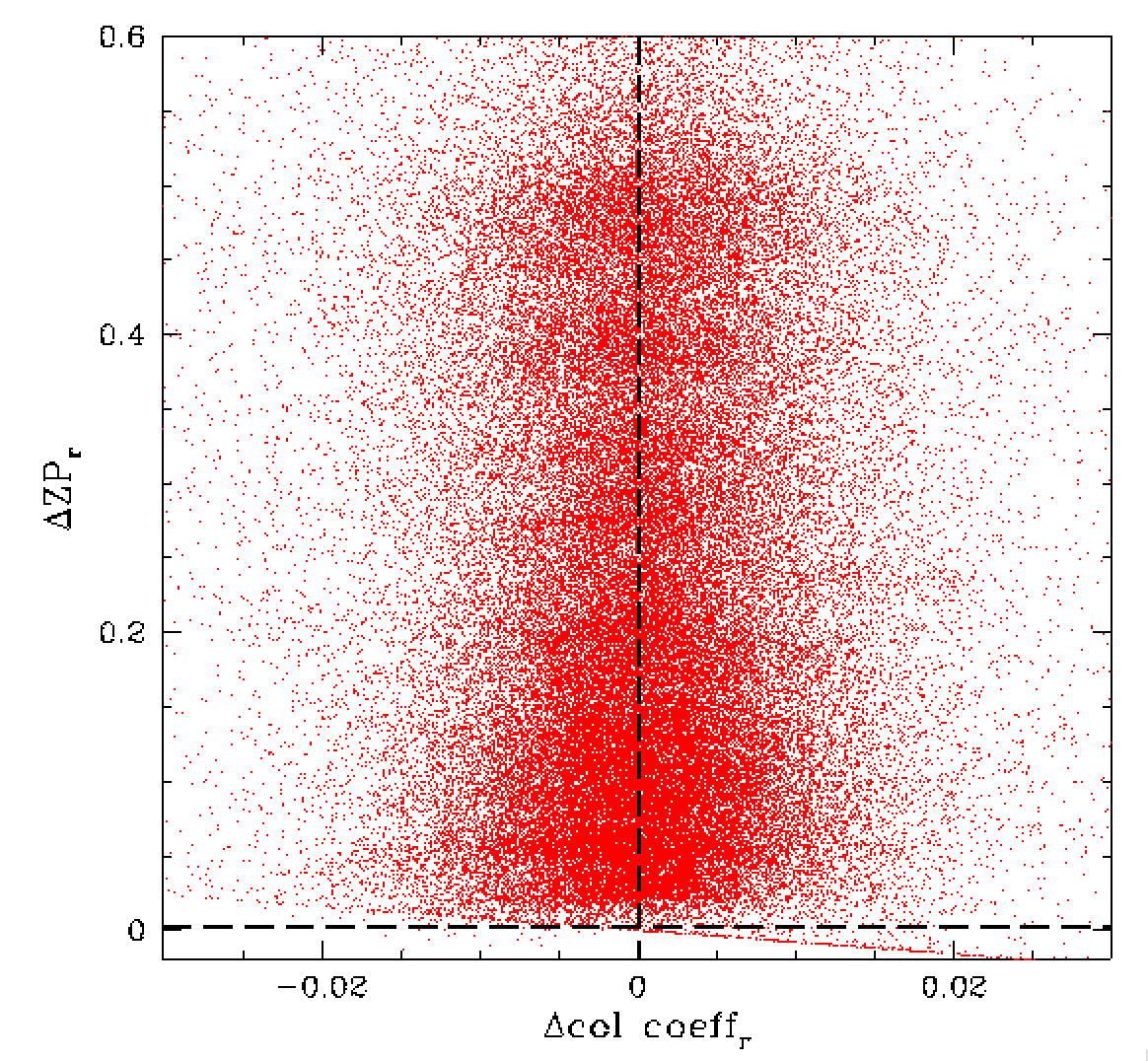
In the left plot above we show the variation in zero points relative to the maximum as well as the variation in the colour coefficient compared to the median determined for a field and tile (for r-band RC0). Here we see that there is a clear trend in ZP values with colour relative to the median for the field, tile, filter combination. This analogus to the trend shown in part 1. Here we see that variations of up to 0.6 mags due to atmospheric extinction are common. Above right, we show the result after adding 0.8 times the difference between the individual measured colour coefficients and the median colour coefficient [deltaZP=0.8x(coeff-medcoeff)].
This correction removes most of the obvious slope in detla ZP with varying colour. Importantly, this demonstates that the observed variation in colour does not scale with the total amount of extinction. That is, the atmospheric components that cause colour changes (i.e. wavelength dependent extinction) generally only cause extinction on limited scale. While the bulk of the extinction (that produces the large ZP changes), is cause by clouds. However, the overall observed extinction is combination of both effects. Thus it may be possible to make an initial estimate for the extinction due to the colour dependent component by looking at the variation between the calculated colour coefficient and the median. The grey component can then be estimated by the remaining difference in ZP relative to the maximum value for a field, i.e. Ext_grey = Zp_max - Zp_model - 0.8x(coeff-medcoeff) where Zp_model is the predicted model value based on airmass, field, time, etc.
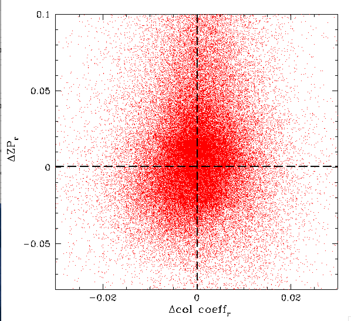
In the plot above we show the zero points relative to the median value for each field (r-band, RC0) after correcting for airmass and the relationship between ZP change and colour change [delta ZP=0.8 x (coeff - median coeff)]. Here we see the intrinsic level of scatter of all the zero points in one r-band quadrant. The 0.05 mag scatter matches our expectation based on the level ZP RMS. However, we will later show that expected distribution is very inaccurate.
Variations in ZP with ZTF field and other parameters
To fully understand why the ZP varies as it does it is necessary to consider which parameters determine the observed zero points. We have already investigated the spatial variation in ZP and systematic variation across the ZTF camera. Here would like to understand how and why the ZPs within a single quadrant vary for between observations and fields so that we can predict the amount of extinction in any given observation.
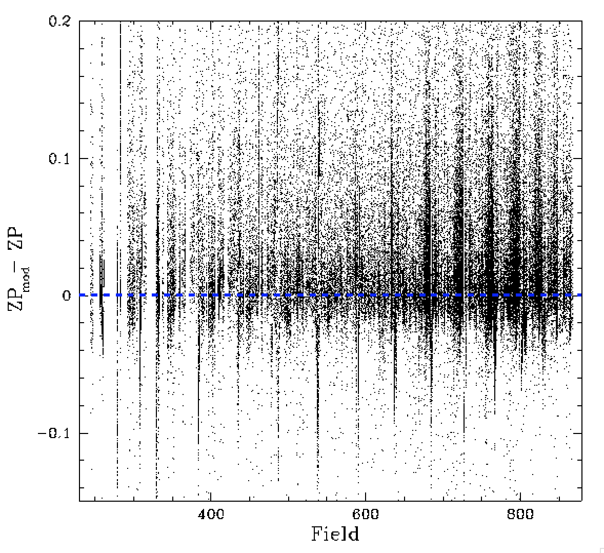
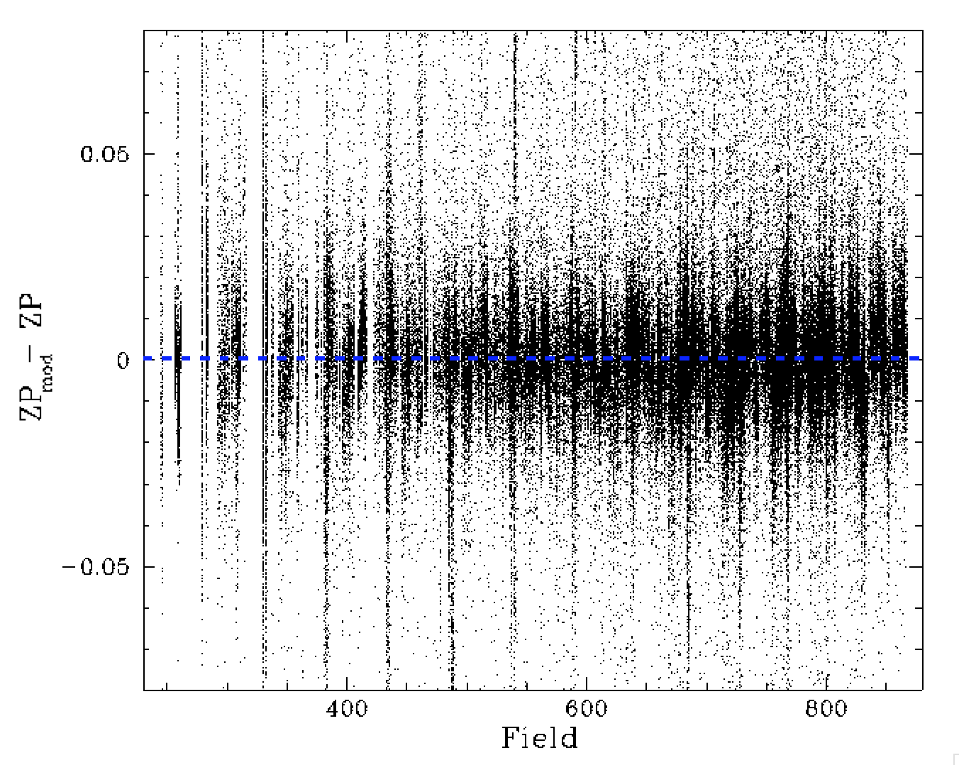
In the plot above we see how the zero points vary relative to their median for different fields (after correcting for the extinction due to airmass [delta ZP_r_air=0.088 x airmass]). Note: we have determined the airmass values used here ourselves since those given in matchfiles, etc., are bogus.
Here we see a clear trend in the range of zero points across each 100 series of fields. These changes are in part due to variations in the colour coefficients (whose values are primarily determined by reddening). Thus, once the colour coefficients are added to the airmass corrected zero points (in the right figure) the amount of structure is reduced. However, even after adding the colour coefficients we still see some structure in the zero points for different fields.
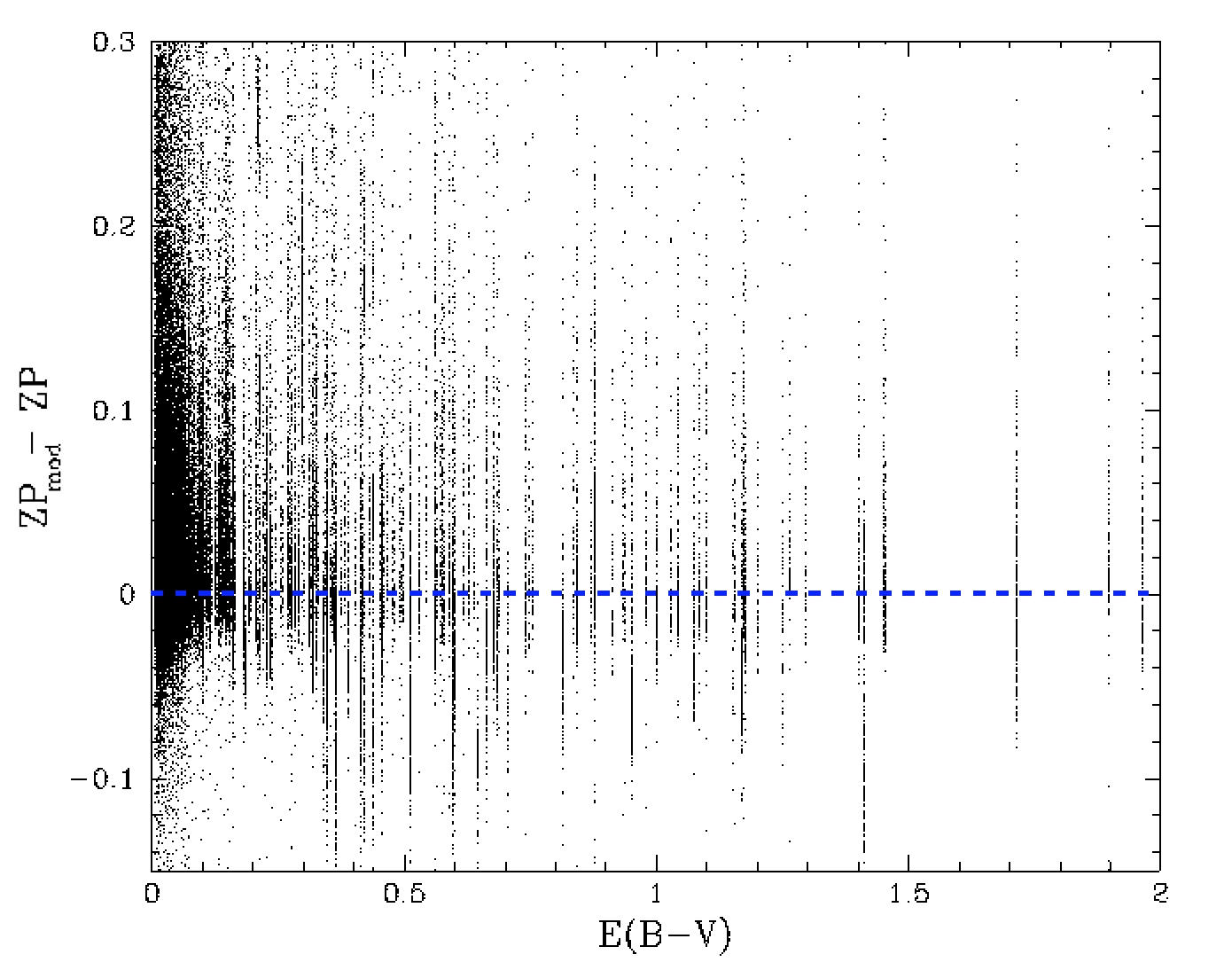
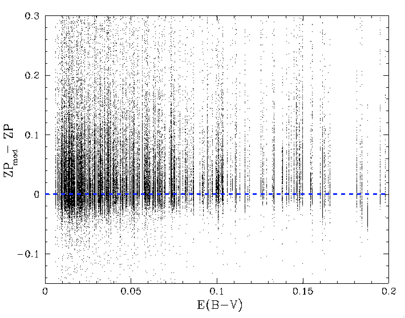
Since field reddening mainly determines the colour coefficient it is worth investigating the in influence of field extinction. We determined E(B-V)values for every ZTF field and quadrant since those given elsewhere are also bogus. After adding the colour coefficients to the zero points we noticed a residual trend in the zero point for high reddening values. The additional of a small (0.008*E(B-V)) term corrected this. However, the left plot above shows that the zero points of field with E(B-V) are offset. Thus an additional reddending term does not fully explain the residual structure in ZPs by field.
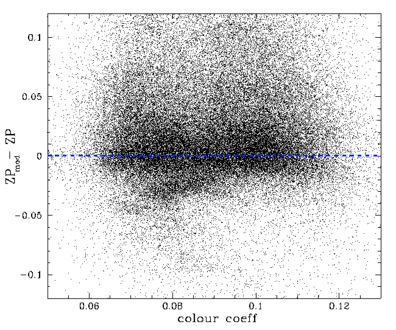
Since both ZPs and colour coefficients are fitted during calibration process it is useful to look at the difference between our our airmass, colour coeff and reddening ZP model varies with colour. In the above plot we show the fit colour coefficients vs the corrected zero points. Here we found that the reddening correction reduced the scatter slightly. However, a region of colour coefficients between 0.075 to 0.095 (which match moderate reddening) was present where the ZP model poorly matched the observations.
Time Dependence
Clearly there is an expectation that the photometric zero points we measure will change over time. For example, from our prior work we know that dust builds up on the optics reducing the overall throughput.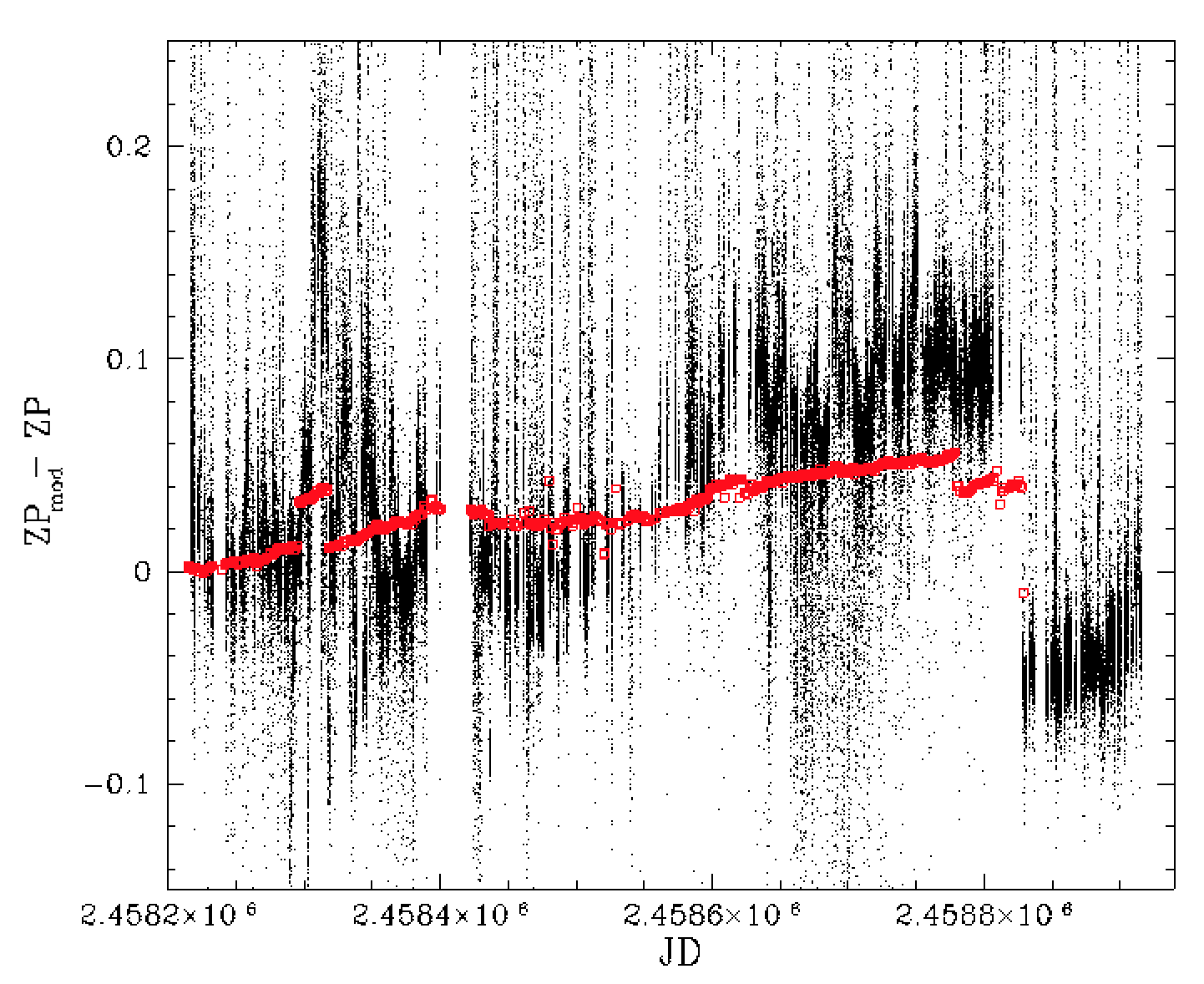
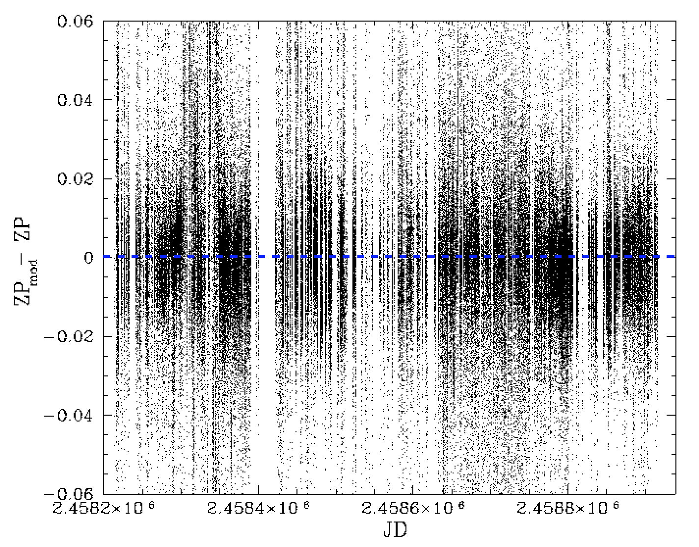
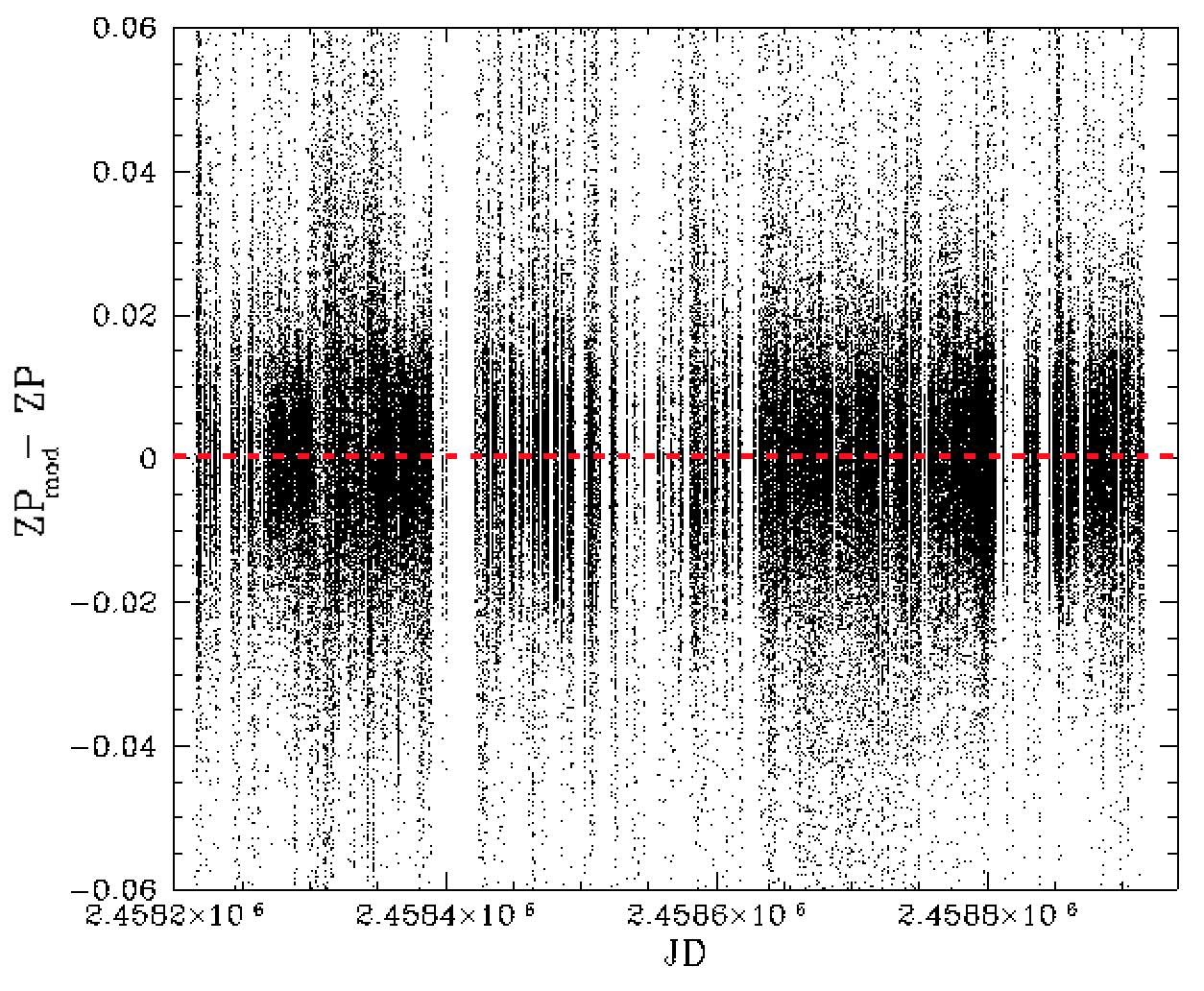
Variations in ZP zero point for r-band RC0 versus the observation date. The red boxes give the variation in measured flatfield median values over the same time period.
When we look at the evolution of the zero points over time we see very significant (~0.2 mag amplitude) structure over the span of ~2 years of observations (2458200 = 2018-03-24, 2458910 = 2020-03-01). Some ZP structure is expected due to cloudy nights as well as the dust acculation. For example, we expect weather will change observed zero points seasonally.
Many of the ZP variations that can be attributed to the instrument are shown by the variations in the flatfield median values (in mag). For example, the change on 2458827 (December 10, 2019) is directly related to cleaning of the telescope optics. However, the observed ZP change on this date is at least twice as large as expected by the variation in 4.7% flatfield illumination.
Our expectation is that the variations in flat field medians should be a close match to overall variation assuming that the illumination level has not varied significantly. Our prior work suggests that these are generally stable to 0.2% between nights with some larger variations due to cleaning or acculation of ash from fires. The reason that the observed ZP changes are so much larger than expected from flats is unknown.
Another feature of this data is that there are clearly many images where with ZPs less than zero. This was completely unexpected since it suggests that a small number of images are deeper even though we have only selected images with 30 second exposures. From the upper plots above we know these match fields with moderate reddening values.
The next step in this process is to model the structure due to the variation in the instrument over time. From the figure above it is clear that there is a strong band of ZPs. We believe these are the baseline lowest extinction observations that reflect real variations in the instrumental throughput. Above this band there is a cloud of lower ZP values due to the presence of varying extinction during a night. On some nights there is no lower band since all of the images were taken through clouds.
Since the distribution on each night is generally skewed with a long tail, this suggests that neither the means, nor medians, will provide a good estimate for cloud-free band of values. Likewise, the presence of negative values shows us that the maxima are also not a good estimate of cloud-free measurements.
In order to trace the main band of observations, we decided to combine the zero points from each image taken on a night assuming that the ZP and ZP_RMS were good approximations for the mean and sigma of normally distributed values. For each night we then found the maxima of these nightly combined ZP distributions and adopt that as our estimate of response.
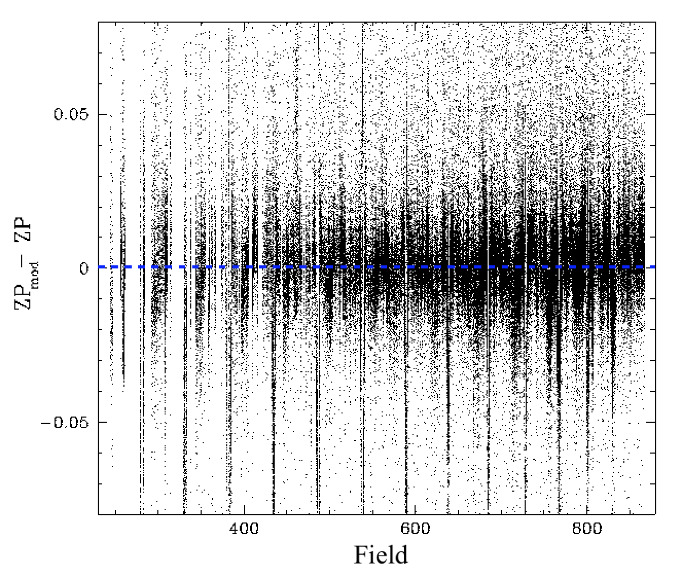
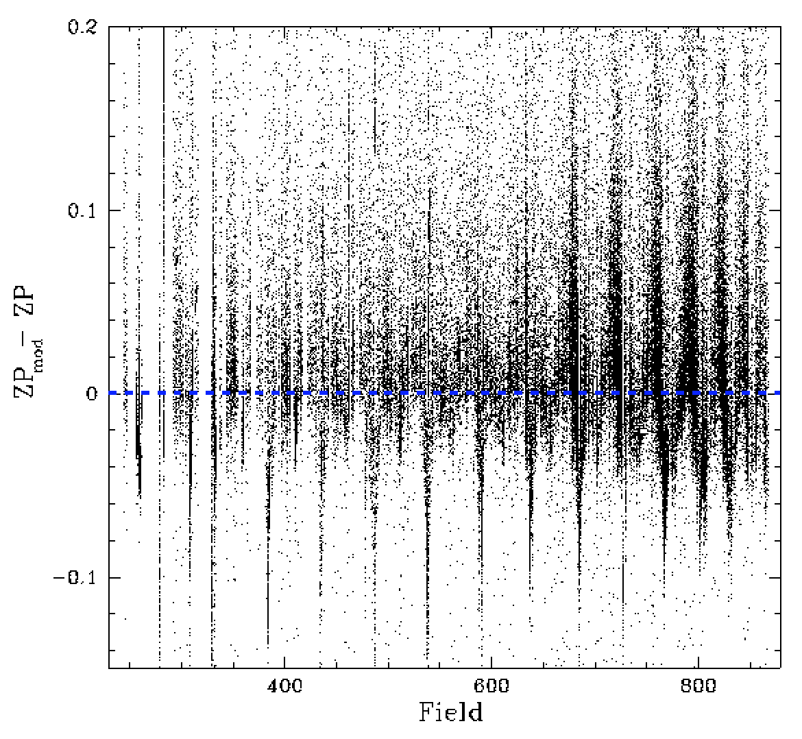
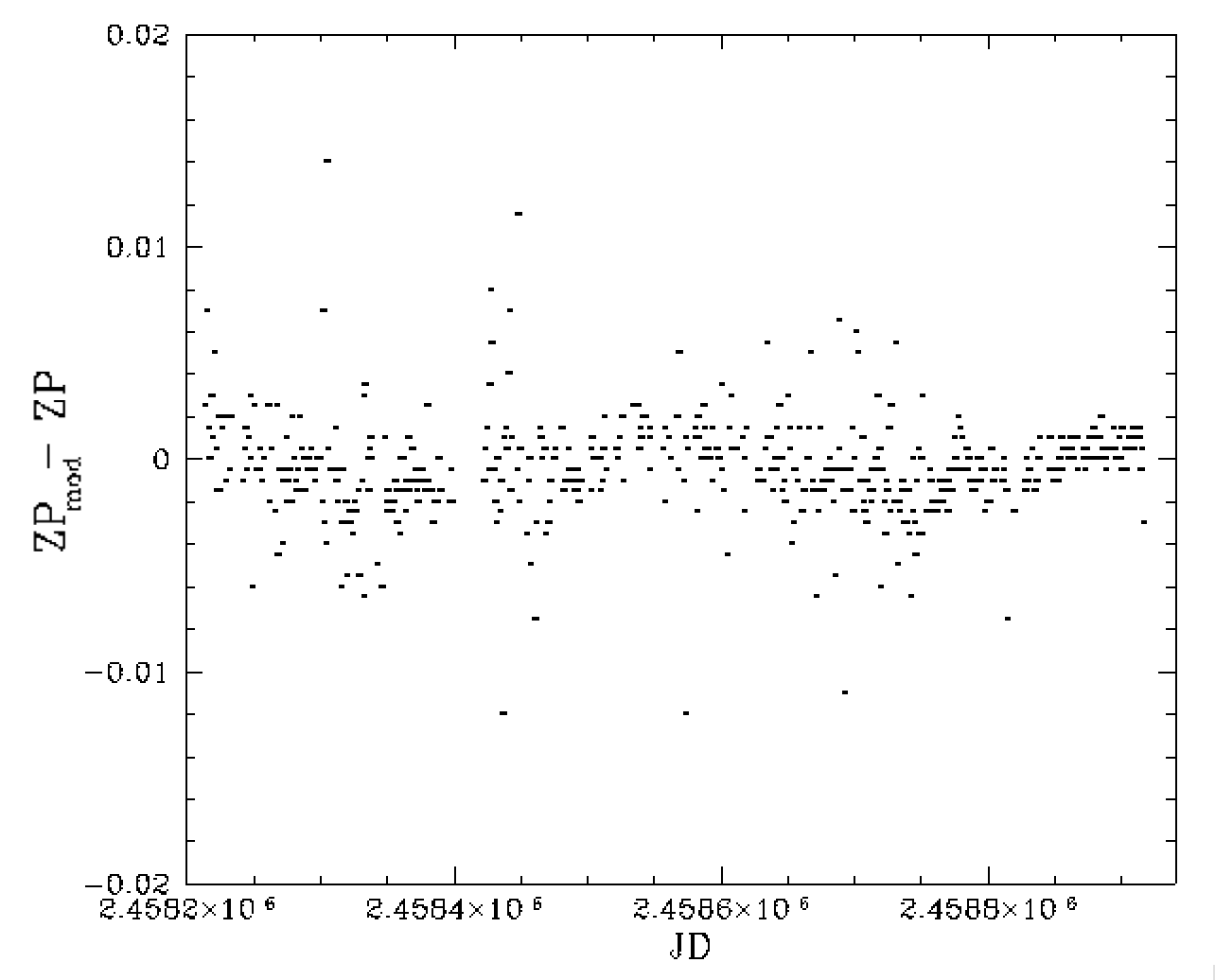
Zero point residuals in fields after correcting for the general trend in ZPs with time.
In the plot above we show the residual trend after removing our time dependent model. Here we see that there are still some trends in the zero point residuals across the different fields. Thus additional terms are required to model the ZP variations.
Trends with the number of catalog sources
From our prior work we recalled that there is a clear trend in the photometric residuals wrt to PS1 with the number of stars used in the calibration, and that the number of calibrator stars depends directly on the number of catalog stars. Thus it is natural to expect a trend with the number of stars will be present.
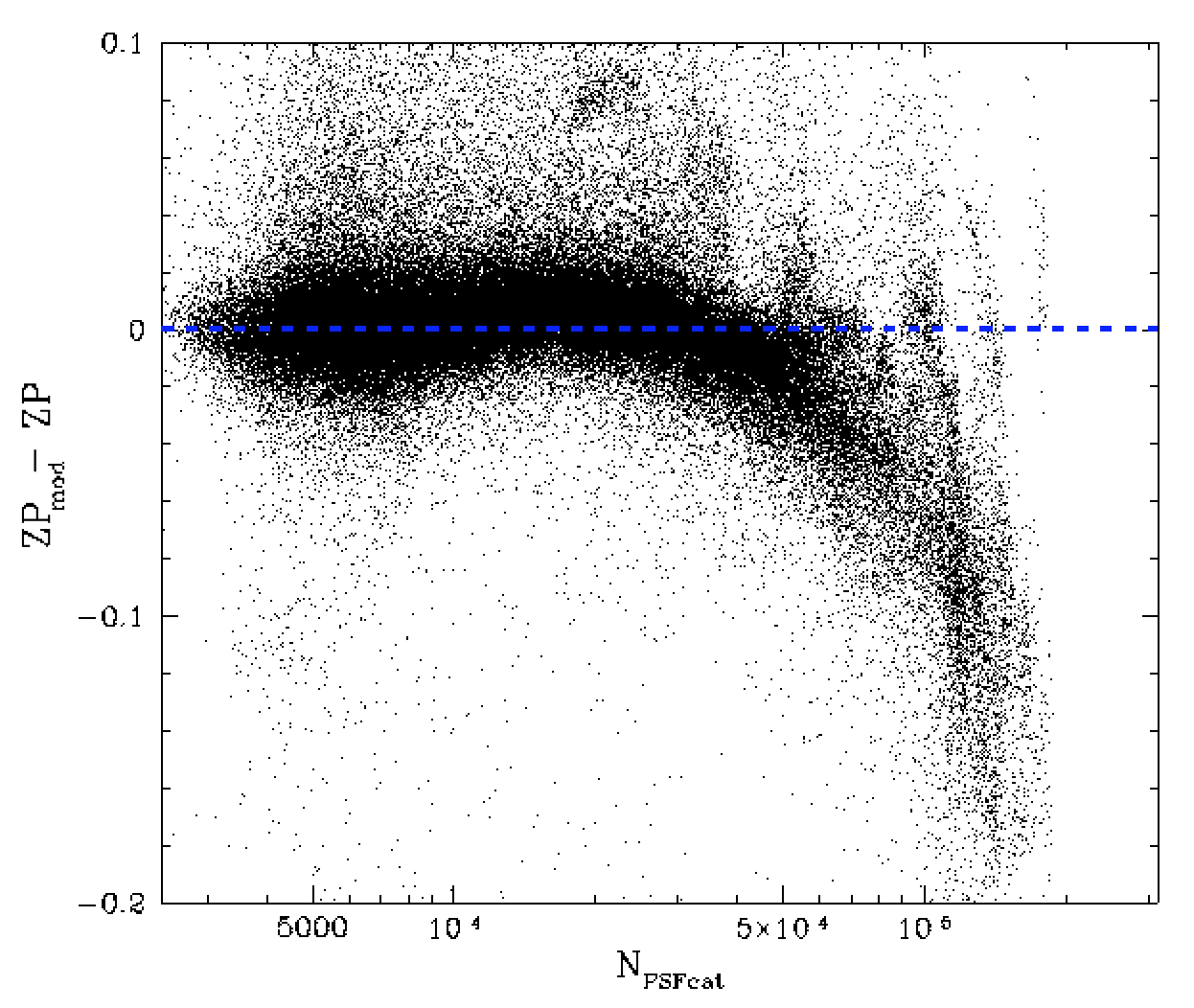
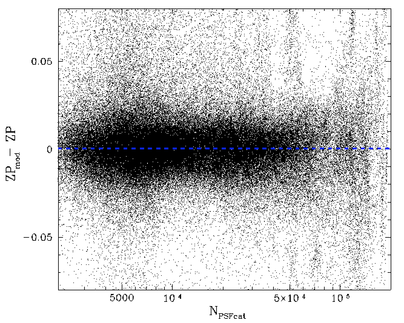
Residual differences between the model and measured zero points vs the number of of calibrator stars within a field.
In the plot above we see that there is a very clear and strong relationship between the number of stars within a field and the measured zero points. We attempted to model this structure with simple polynomial models, but these were insufficient due to small scale strucure even when we clipped outliers. We eventually binned the data and fit a spline to the values. In the right plot above we show the residuals after subtracting the spline fit. For large number of catalog stars the model is poorly constrained.
Trends in residual zero points with field and observation date after removing the field density trend.
In the plots above we show the result of removing the trend with the number of catalog sources (a source density effect). The resulting plots still exhibit structure. The problem here is that, when the trend with time that was first determined it included the source density effect and thus biased the nightly results. Thus we recalculate the time dependence after correcting for the source density trend.
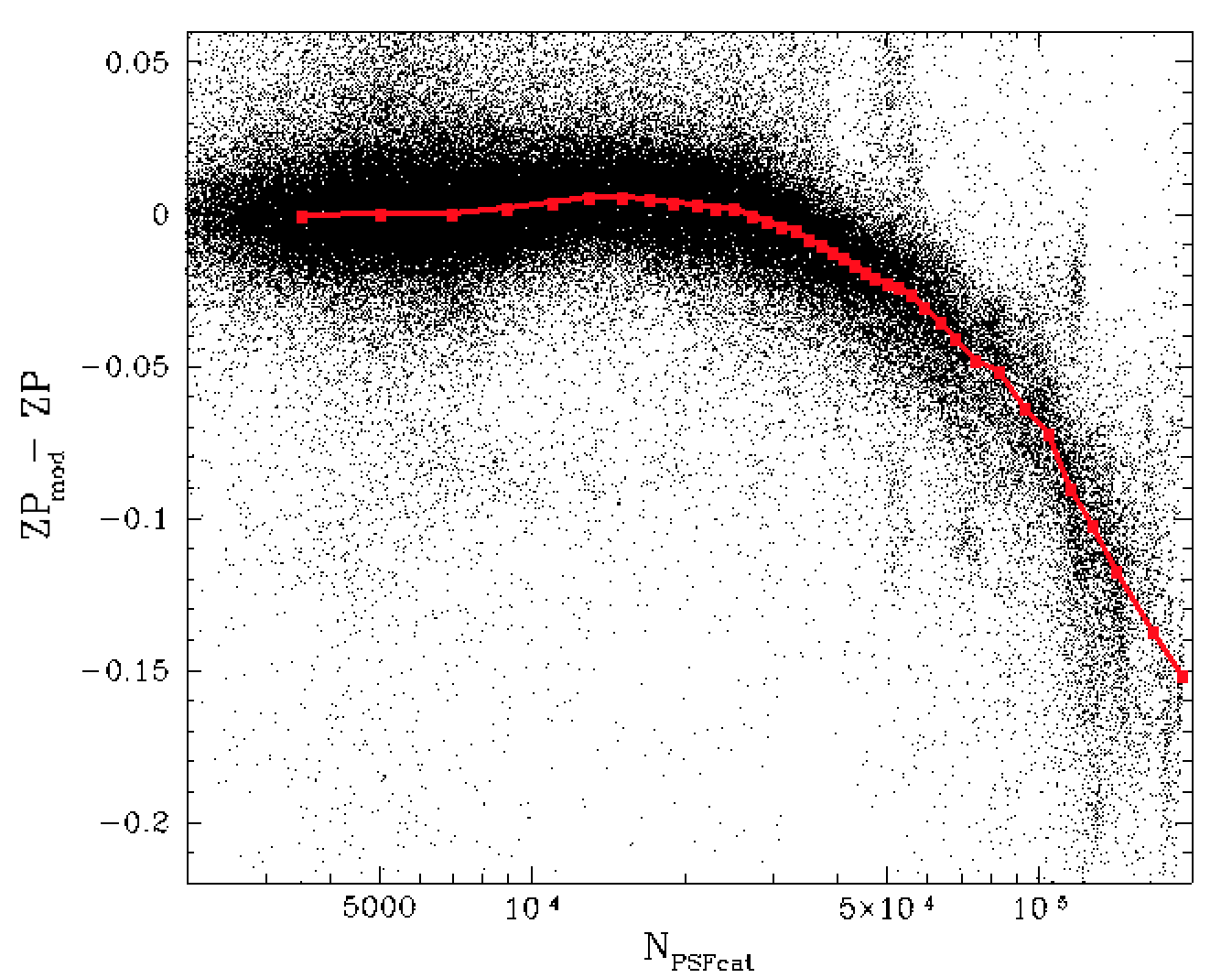
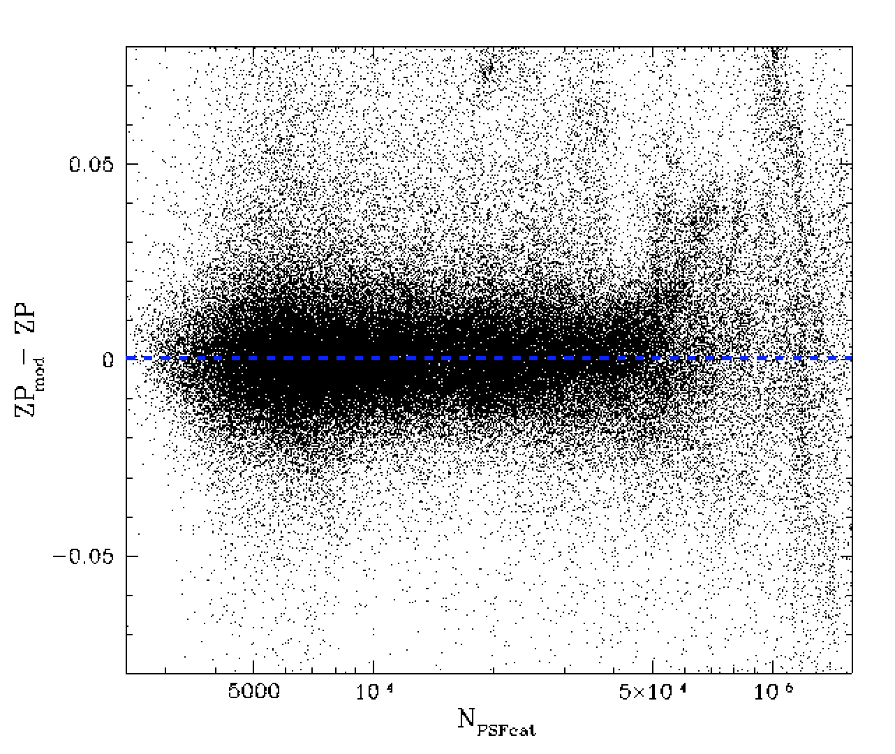
Residual differences between the model and measured zero points vs the number of of calibrator stars within a field after removing time dependent trend. The red line is the spline fit to the trend.
We then recalcuate the source density dependence again. The results source density trend is now cleaner. Once again we determine the trend with time after removing the new estimate of the source density dependence.
Trends in residual zero points with field and observation date after removing the improved estimate of the field density trend. The right plot shows how the estimates have changed.
In the plot above we see that the structure across nights has largely been removed by our iterative determination of the source density dependence. In the right plot we show the effect of this iteration process by plot the change in the nightly zero point model. Interestingly the result is sinusoidal and may relate to the season variations over 2 years.
Field Offsets
In earlier work we discovered that ZTF fields calibrated to PS1 exhibit distinct offsets relative to other fields. The reason for these offset is unknown, but may relate to variations in populations of calibration stars. These trends are very small and thus unclear when looking at all fields together.
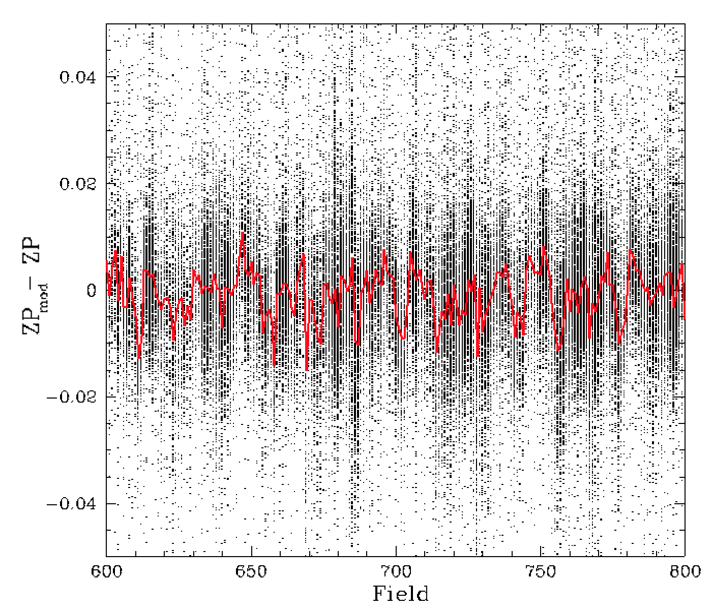
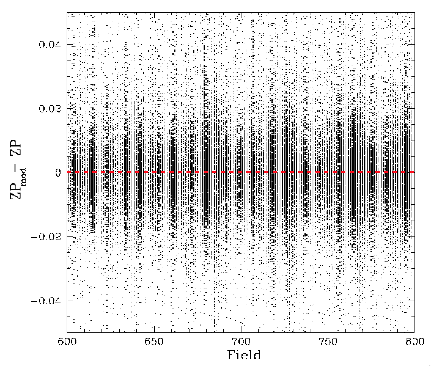
Trends in residual zero points with field and observation date after removing the improved estimate of the field density trend. The right plot shows how the result of removing field offsets.
When we zoom into the ZP residuals for a small number of fields we can clearly see that there are variations between each field (as expected). Following the same process as our time-dependence determination, we find the peak density of residual ZP for each field and remove this as shown in the right plot above. The result is now free of obvious structure apart from varying spread between field, which is due to variation in the uncertainties with the number of calibration sources as we saw in part 1.
The RMS difference between the final ZP model (involving airmass, colour coefficient, field density, time trend and field offset) and the fitted ZPs is 1.0%.
Checking ZP Model Dependencies
As a check for any remaining dependencies we plotted the ZP residuals versus and number of other observational parameters that often affect them.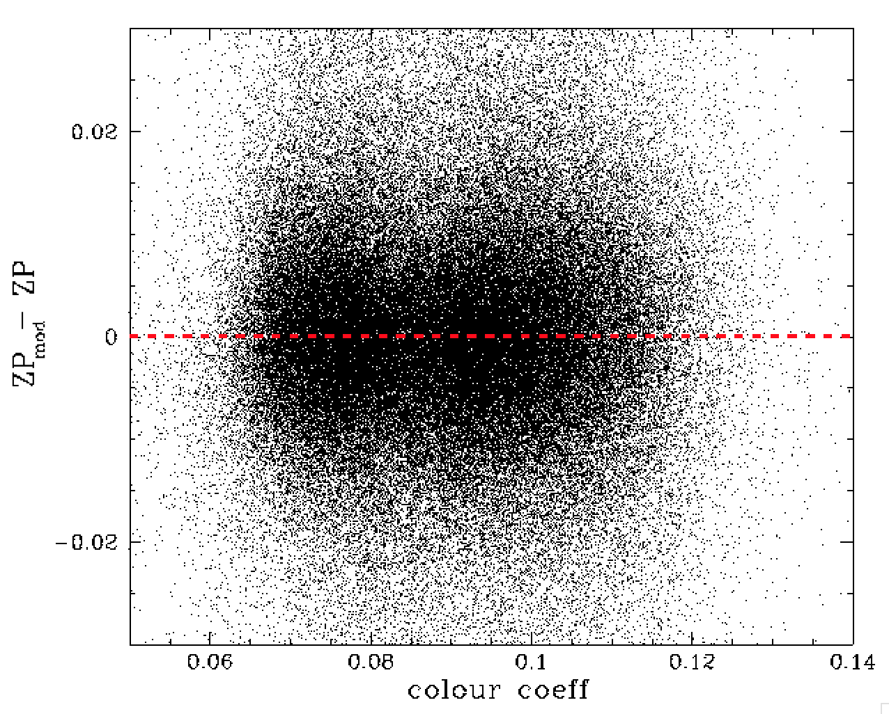
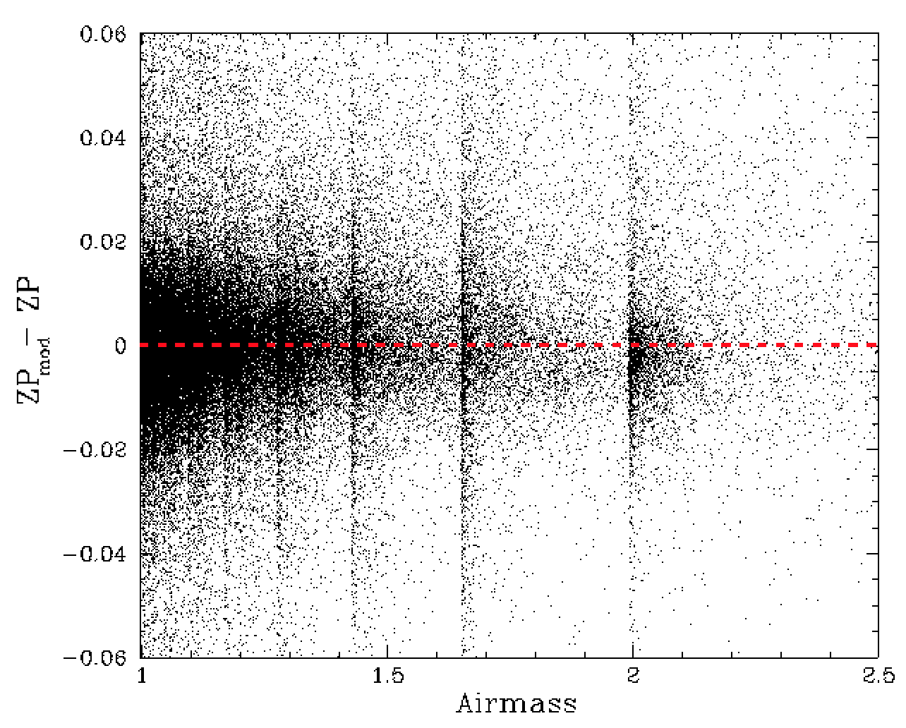
ZP model residuals vs colour coefficients and airmass.
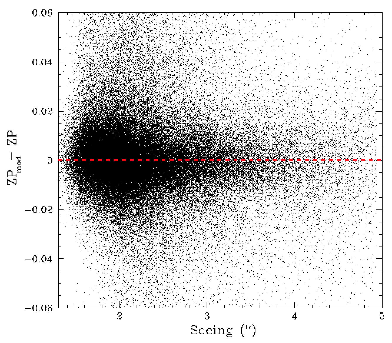
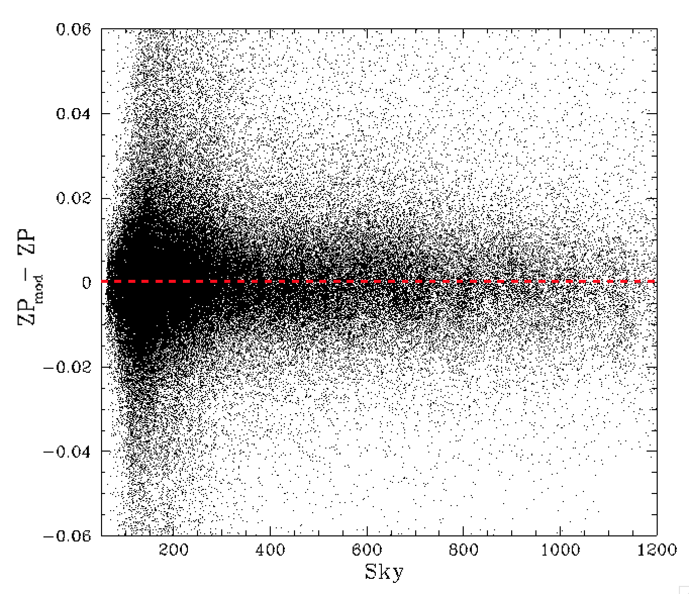
ZP model residuals vs seeing coefficients and sky background level.
We find no obvious structure in the ZP residuals relating to colour coefficents, airmass, seeing and sky level.
Other Noteworthy Trends
Given the large set (~160,000) of ZPs (and related paramaters) we compile for a single quadrant, it is worth checking for other relations that might affect the calibration. Thus, we also investigated other trends within the data.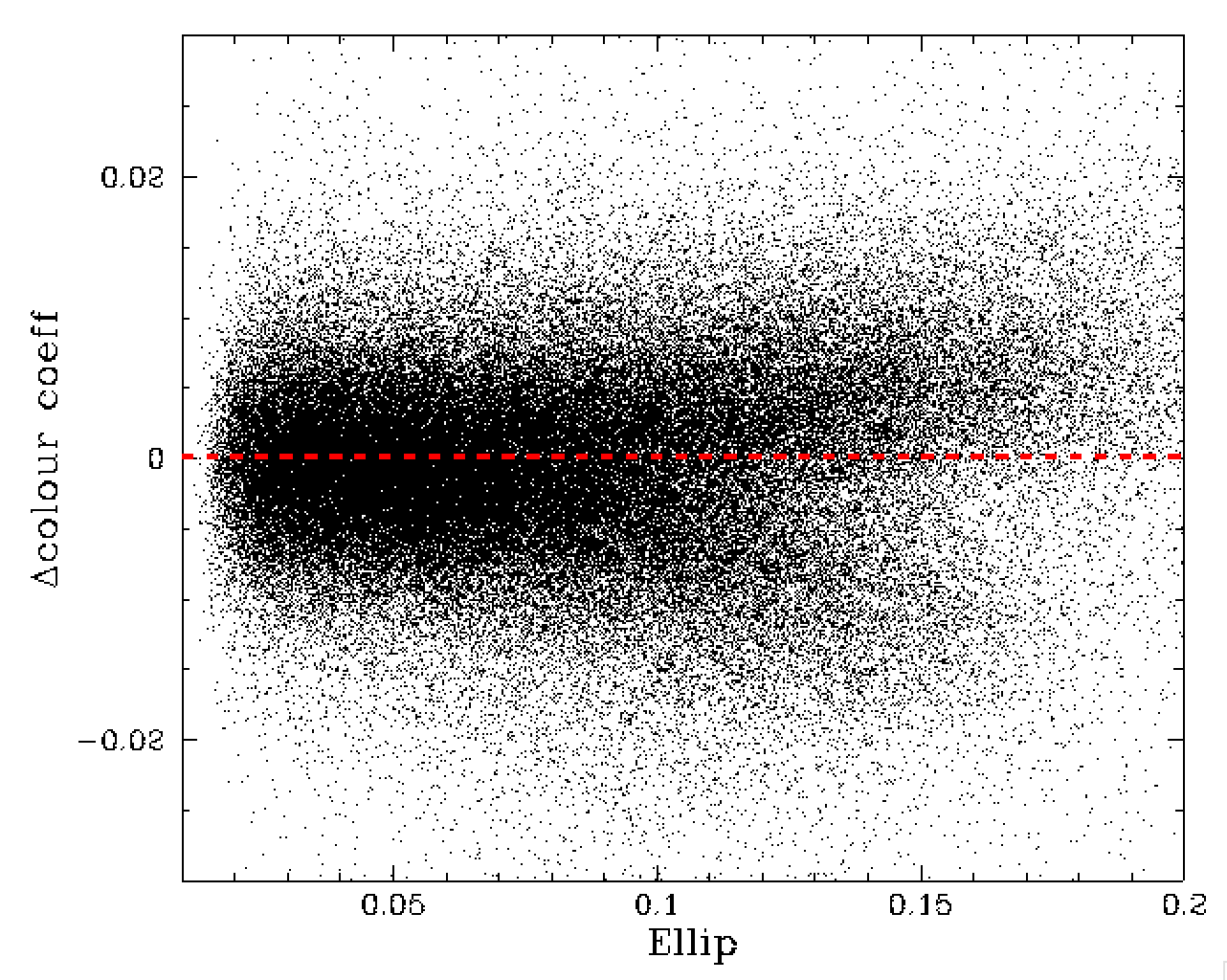
Average ellipticity vs variation of the colour coefficient from the median value for a field.
In the plot above we see that frames with large values of average ellipticity are associated with deviations from the median colour of a frame. This may be a sign that poorly focused frames have systematic errors in their colour coefficients.
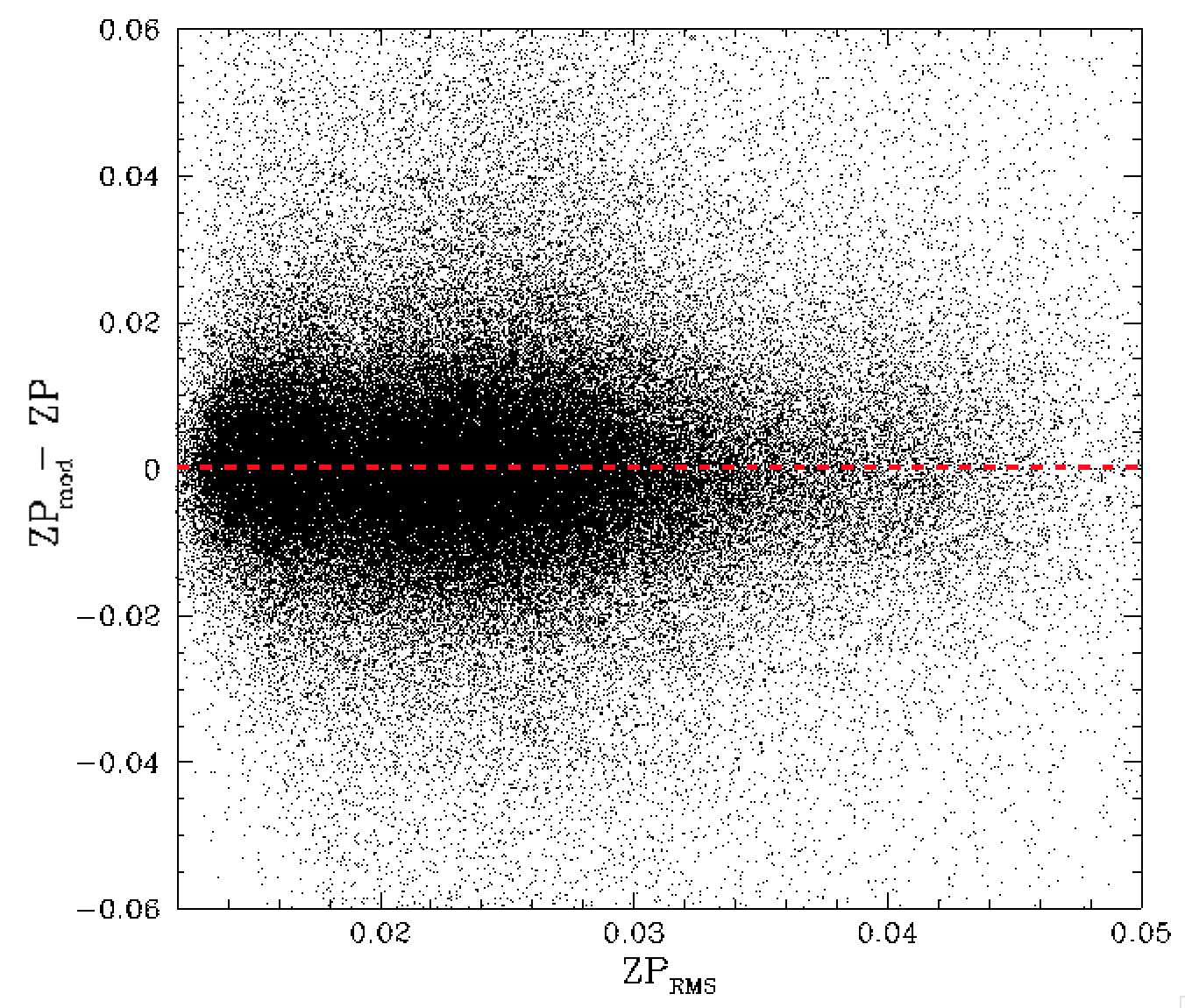
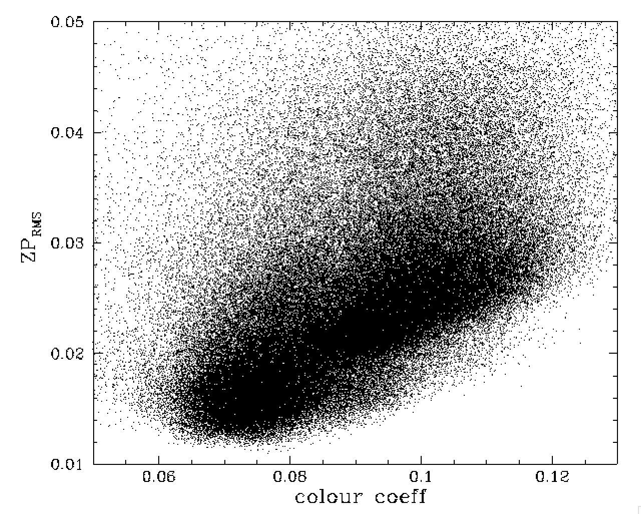
ZP model residuals vs ZP RMS and colour coefficient vs ZP RMS.
In the plot above we see that the scatter from our ZP model is poorly correlated with the expected scatter based on the value of ZP RMS from fits. This suggests that the ZP RMS values in many frames is overestimated (indvidual field photometry also suggests this). One possible cause for this correlated errors. The righthand plot above we show that the ZP RMS values are strongly related to the values of colour coefficent.
As previously shown, this is most likely relates to the fact that fields with blue colour coefficients include many bright foreground stars, while those with red coefficents are highly reddened and use faint red stars. However, this does not explain why the values are larger unless the correlation relates to the fact that the terms are fitted together and are an incomplete model of the physical situation.
Lastly, the model above does not include the dependency on measured star colours on airmass. The distribution of colour coefficents do not show any relationship with airmass since the colour coefficient are dominated by reddening in r-band. However, when we determine how the colour coefficents in a field change relative to the average airmass, we do see a small but clear trend as shown below [colour coeff - median colour coeff = 0.0079*(airmass - average airmass)]. Include this term in the model reduces the residual scatter to 0.99%.
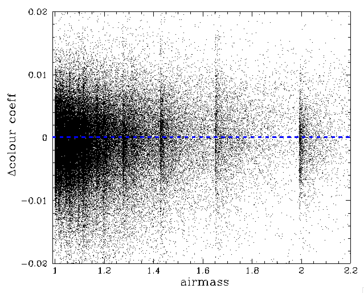
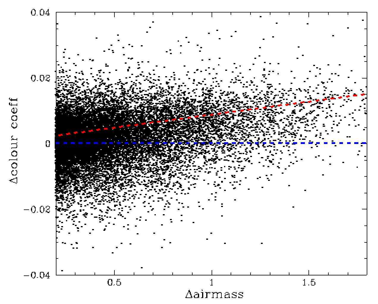
Variation of colour coefficient relative to the median for field vs airmass and the change in airmass from the average for that field. The line red dashed-line shows a slope of delta colcoeff = 0.0079*(airmass - average_airmass).
Conclusions
We have created method to model the ZPs in each ZTF field and frame in order to determine the amount of atmospheric extinction in each observation. This model uses the current ZP and colour coefficient fit values, but can be modified to give slightly less accurate values based on medians for each field. The current model appears to provide extinction-free estimates accurate to 1% and is based on airmass, obs date, crowding, etc. Furthermore, although the current method has only been applied to a single r-band quadrant, it should work for all quadrants and filters. The model also relies on having at least a few measurements during a night without significant atmospheric extinction. This wont be the case for some nights. However, these nights can be flagged based on the scatter in their nightly ZPs.Although the aim of the model is to determined extinxtion estimates within the Zubercal single night calibration process, an additional benefit is that such models will allow us flag bad data based on their deviation from an expected value. i.e. we can flag individual images using extinction (outlier) estimates without making general cuts that might cut good data or keep bad data.
The current analysis highlights a few unexpected results:
1, The ZP RMS values from fits do not appear to accurately
reflect the ZP uncertainties (this may have a slight affect on
our time-dependence determination above).
2, The systematic variation in zero points over time is much
larger than expected based on the levels observed in flatfields
which are epxected to provide constant illumination (and do
on short timescales).
3, The presence of a systematic variation in ZPs between fields
remains to be explained.
4, The trend of increasing ZPs with increasing source density
is counterintuitive since it suggests we go deeper in crowded
fields where blending should limit our depth.