| Topics |
|---|
| Modelling g-band zero points. |
| ZP stellar density dependence. |
| Field Offsets. |
| Checking Results. |
| Conclusions. |
Motivation
In part 1 we started exploring the Uber calibration of ZTF photometry and discovered that this process requires understanding of both atmospheric extinction as well as variations in the throughput of the telescope.In part 2 we modelled the variations in ZP for an r-band quadrant.
Here we will do the same for g-band.
Modelling ZTF g-band Zero Points
As in part 2 of our Zubercal work we collected all (~100,000) of the all zero points and related parameters for ZTF g-band RC0 primary fields. Images with nonzero error flags, exposures longer than 30 seconds or taken after late March 2020 were not included.
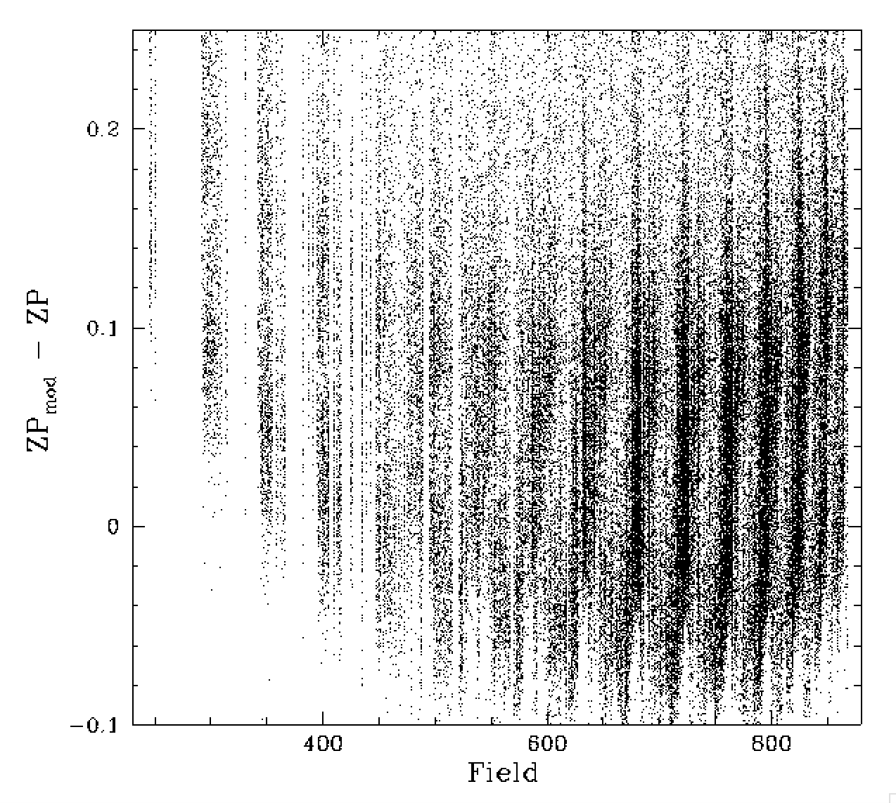
Field dependence of ZTF g-band zero points. Left plot: individual raw ZPs after removing a constant. Right plot: ZPs corrected for a constant and the airmass dependence.
Above we show the initial distribution of zero points before and after correcting for airmass. The plot on the left shows the level of scatter we are dealing with when trying to predict the amount of atmospheric extinction within an observation solely based on a ZP and colour coefficent. Clearly even the airmass corrected ZPs show a lot of structure across fields.
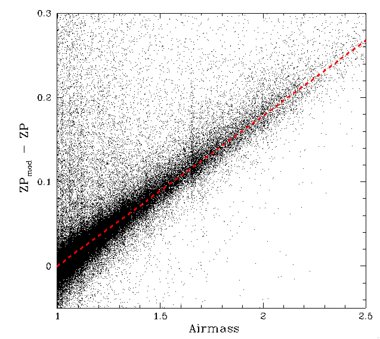
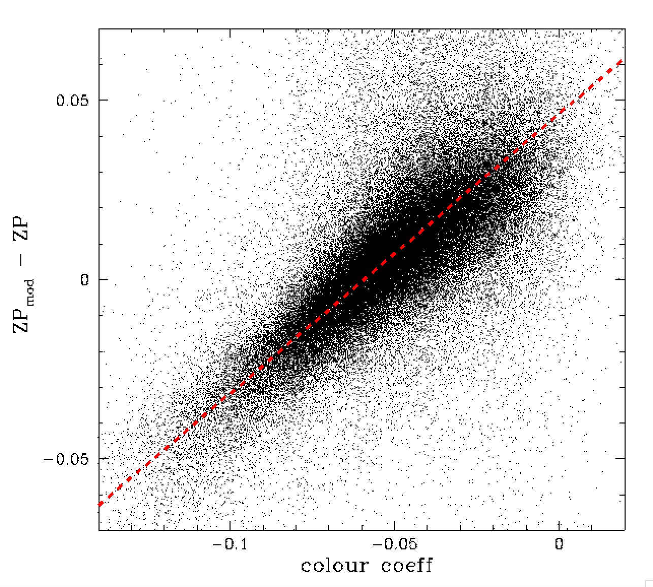
In our analysis we determined that the airmass extinction dependence to be 0.178 mag/airmass (c.f. r-band 0.088). We also found the ZP colour coefficent dependence of 0.78 (r-band 0.82). Plots of these dependencies are given above.
After removing the airmass and colour dependence we determine the very significant time dependence as we did in r-band. That is, we find the peak of the nightly ZP distribution by combining gaussians that have their sigma equal to the measured ZPrms.
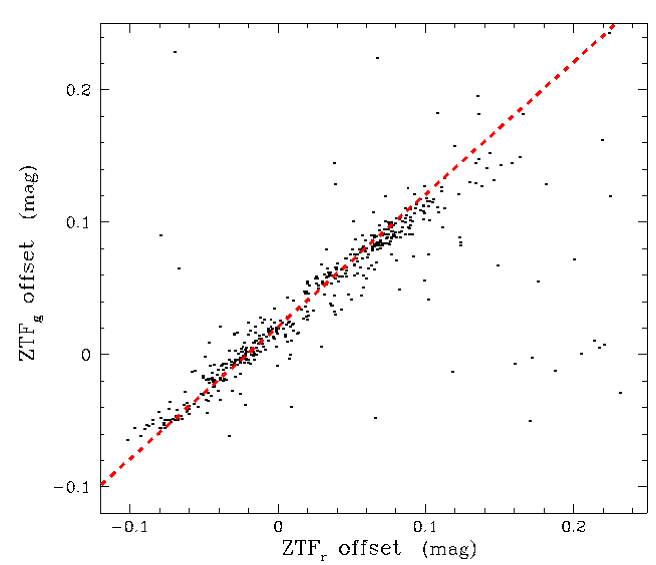
In the right plot above we show a comparison between the g-band and r-band results. Clear the structure us very similar. We also show the offset of the g-band and r-band zero points relative to the model for nights contain both types of observations. Here we see that the slope of the line is very close to 1.0 suggesting that the results are very consistent. The slope of the points suggests there is actually a slightly smaller g-band variation than r-band. The outliers in the plot are due to nights that had few observations as well as those that were affected by clouds.

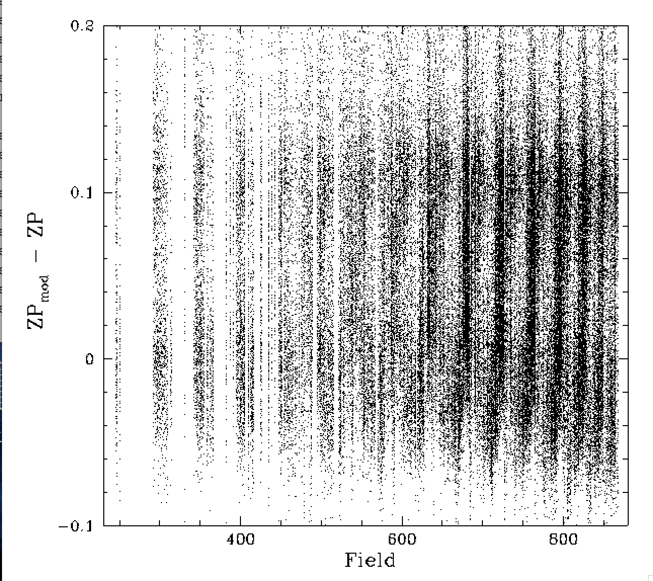
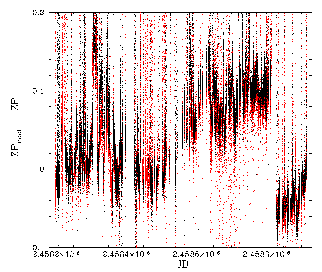
Time and field dependence of ZP model residuals. Left: residuals by field. Right: residuals by JD.
After we remove airmass, colour and baseline time dependence, the ZP data appears quite well modelled as shown above. However, additional terms are required to remove some remaining systematics.
G-band ZP stellar density dependence
The next step in this process was to determine the source density dependence of the g-band ZPs as we did for r-band.

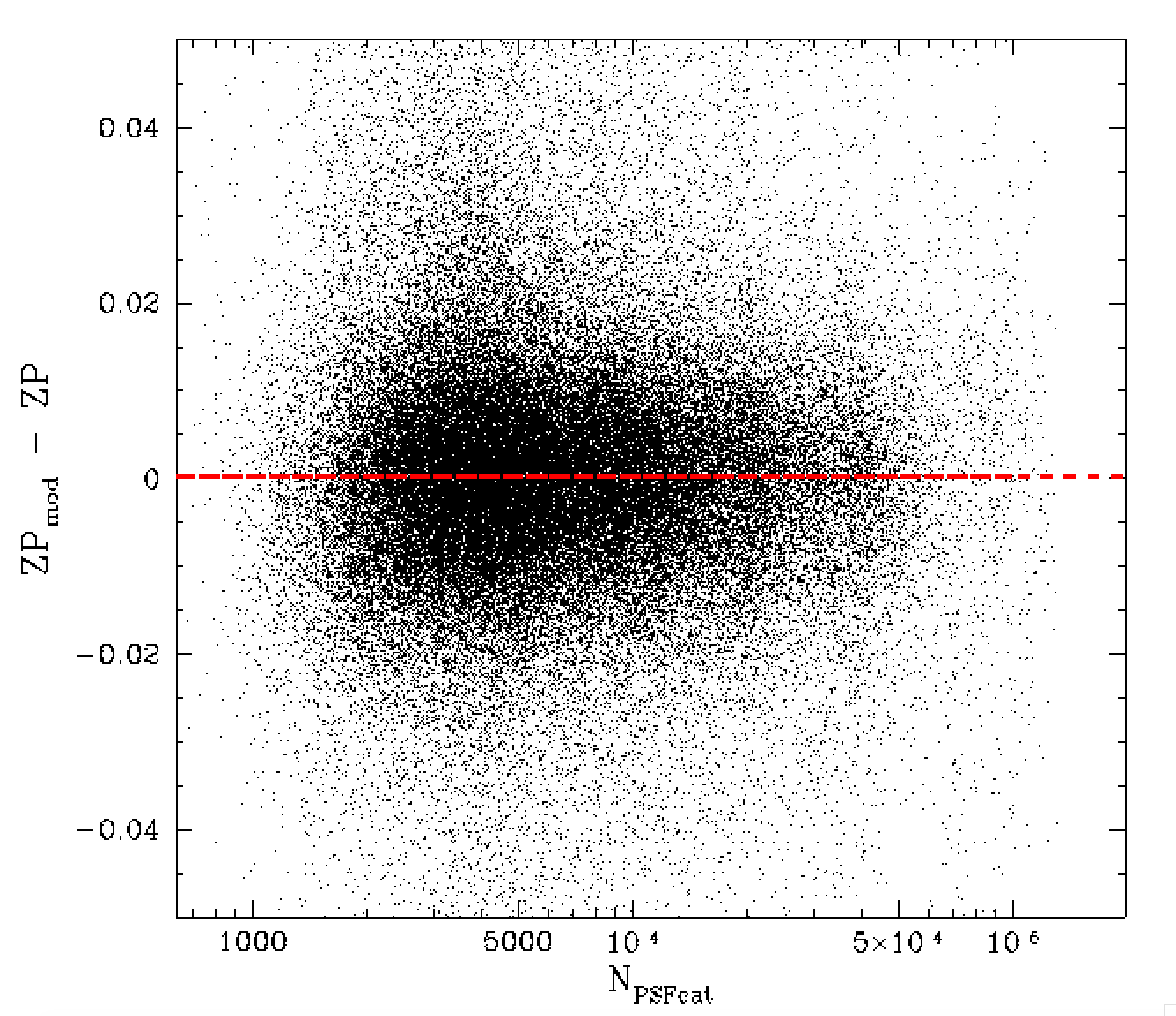
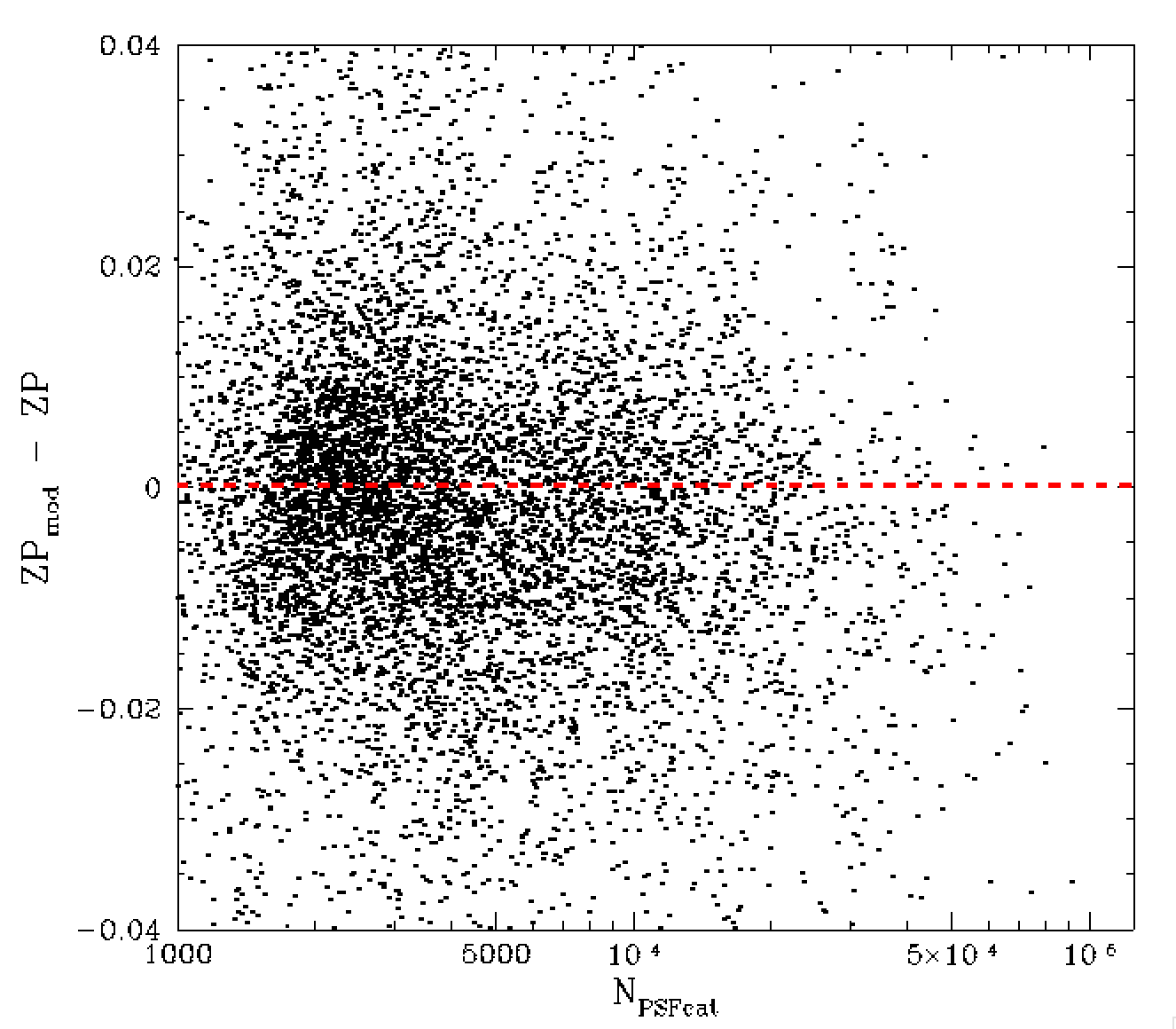
Dependence of ZP residuals on the number of ZTF catalog source in each observation. Left: Original ZP residuals by source number. Right: ZP residual corrected using new source number dependent model.
Here, we once again bin the data based on the number of psf catalog sources and fit the resulting shape with cubic splines. In this case we did not attempt making polynomial fits. The g-band dependence is very similar to r-band. However, they are not exactly the same. The difference is likely due to g-band observations have poorer average seeing than g-band.
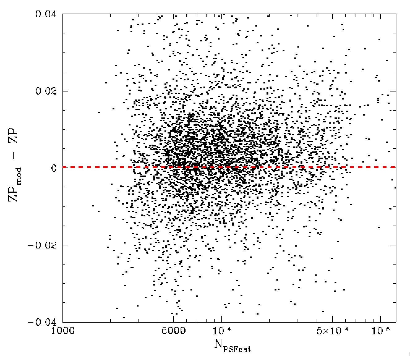
Dependence of ZP residuals on the number of ZTF catalog source and seeing conditions. Left: observations taken with FWHM < 1.8 arcsec. Right: 0bservation with FWHM > 3.5 arcsec.
For example, when we divide observations taken in very good seeing (< 1.8 arcsec) with bad seeing (> 3.5 arcsec) we do see an offset between them (above). That is to say, seeing obviously effects the degree of crowding within images.
Field Offsets
With the airmass, colour coefficient, time and stellar density dependency determined the next step is to calculate field offset as we did for r-band.
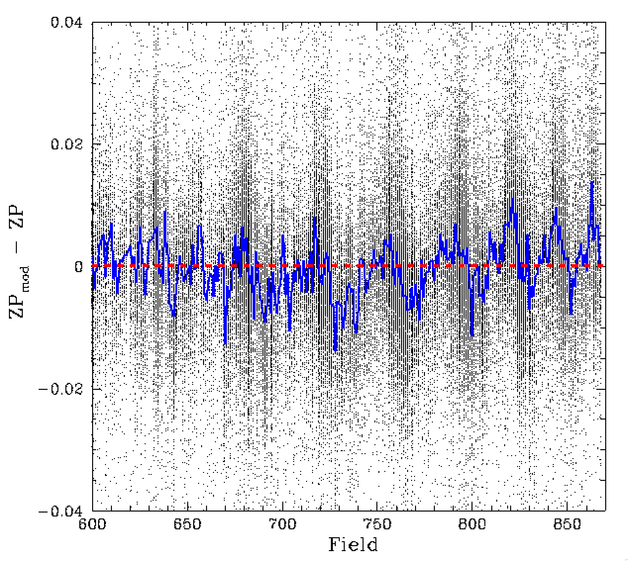
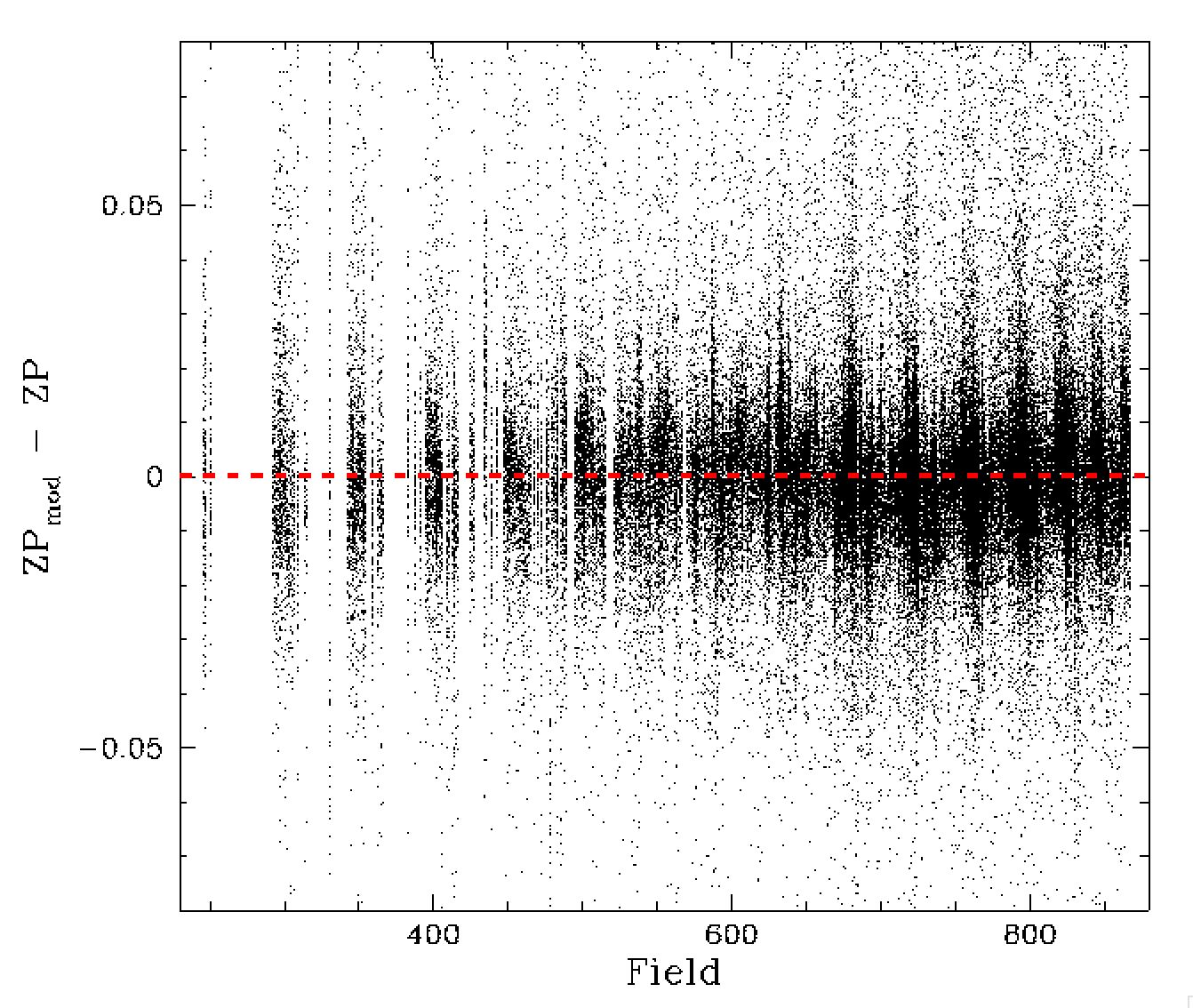
Variation of the zero point residuals by field. Left: dZP residual distribution before removing offsets. Right: residuals are removing field offsets. The blue line connects the peak residuals for each field.
Once again this is done by assuming each measured ZP can be approximated by a Gaussian with mean ZP and standard deviation equivilent to ZPrms. The peak density of the combined distribution give us the offset for the field relative to the model. The results are given above. The field offsets show a very clear structure. Such structure was evident in our earlier work which suggested a link with Galatic latitude.
The resulting residual difference between the model and fits has an RMS of 1.2%. This is slightly large than r-band and expected given that g-band has more spatial structure and few calibrators.
Checking For Additional Dependencies
After modelling how the g-band zero points vary with the most important parameters we then look for any remaining dependency among them.
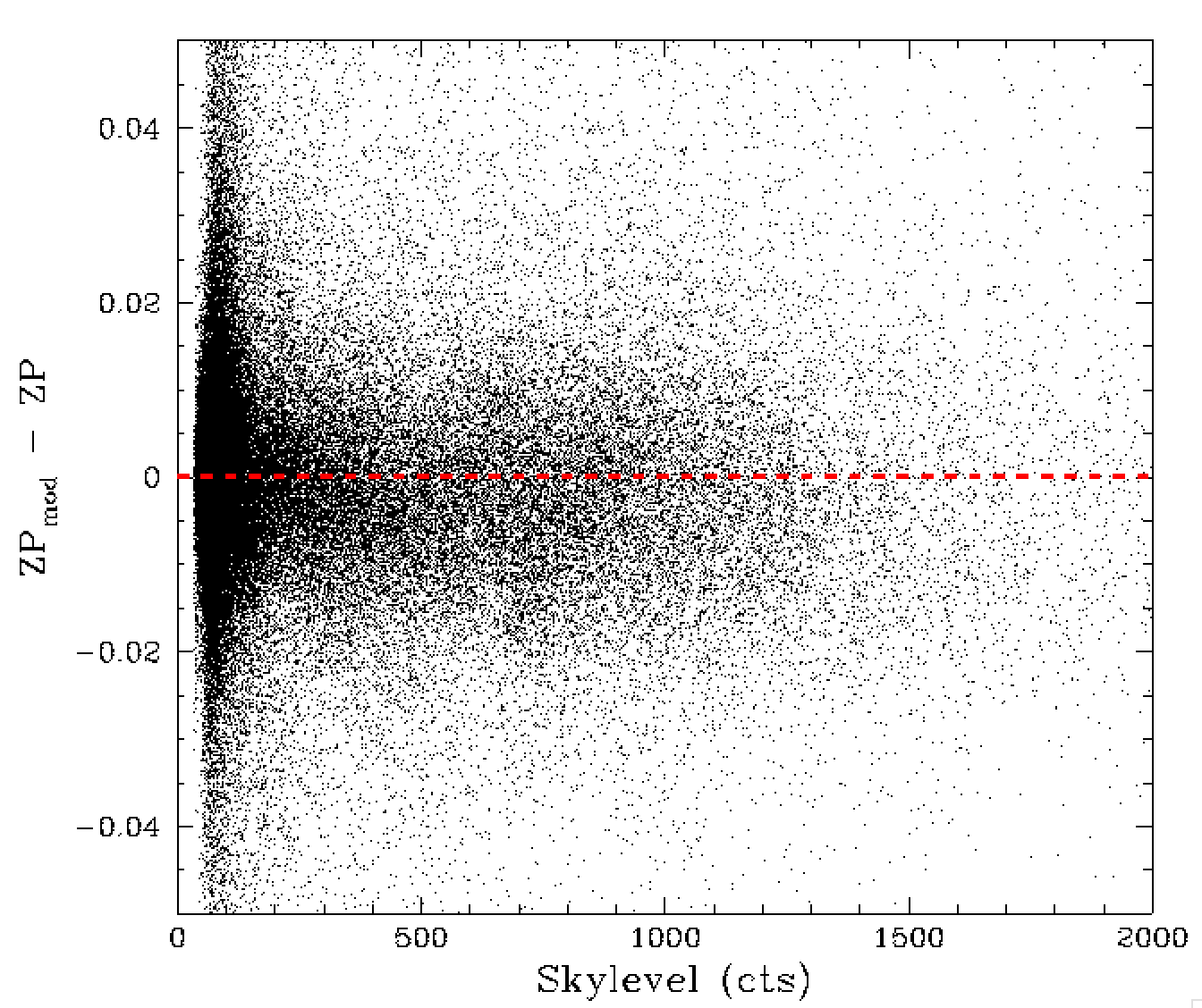
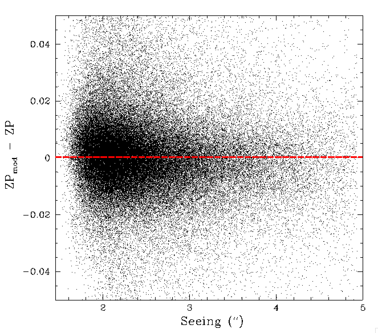
Residual differences between ZP and the ZP model for values sky and seeing.
Above we show the skylevel and seeing dependence of the ZTF model ZPs. Notably there is no clear trend in ZP residuals with skylevel, while eariler we found a strong trend in sources residuals with skylevel. This is most likely due to the source crowding effect being removed.
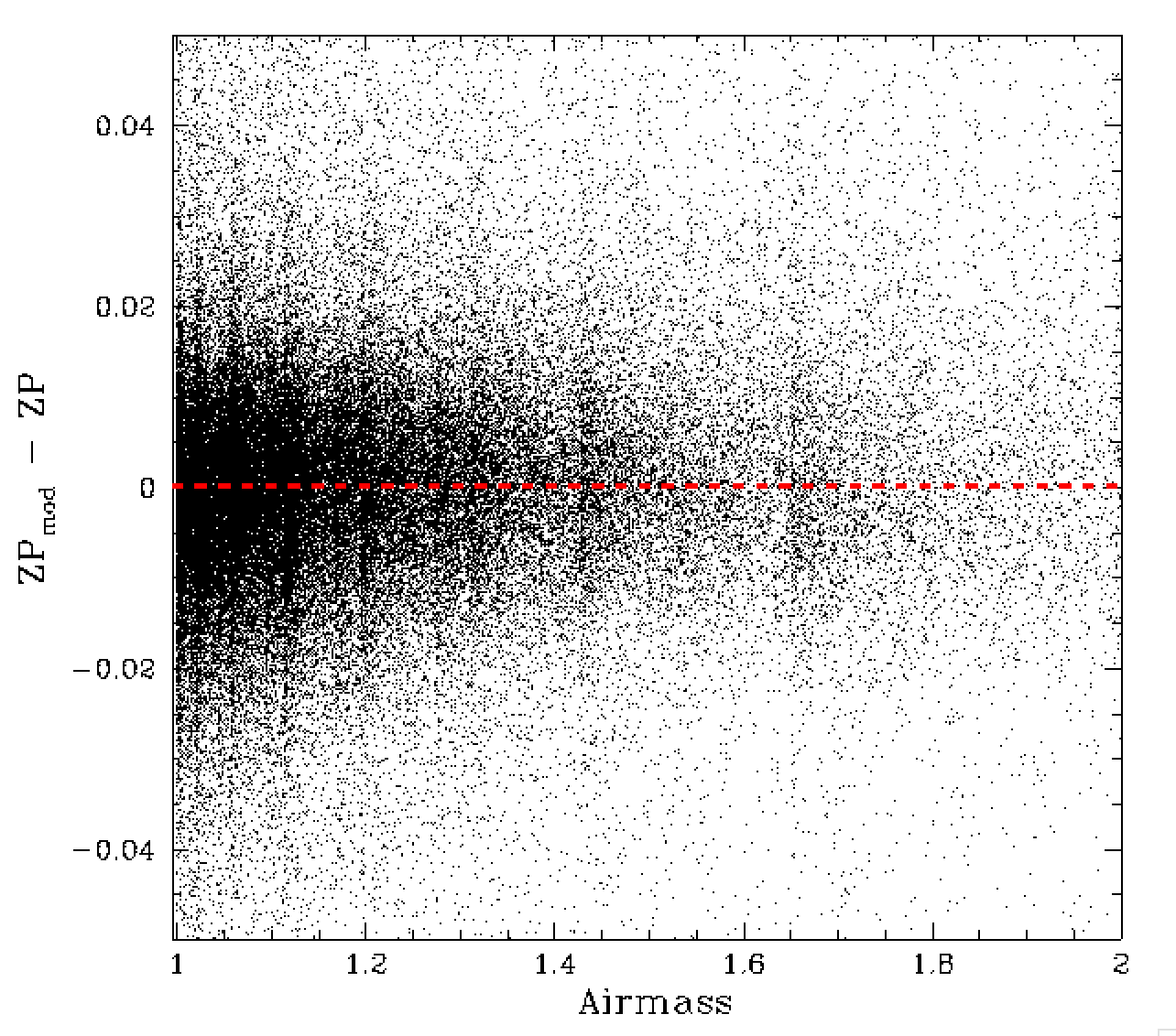
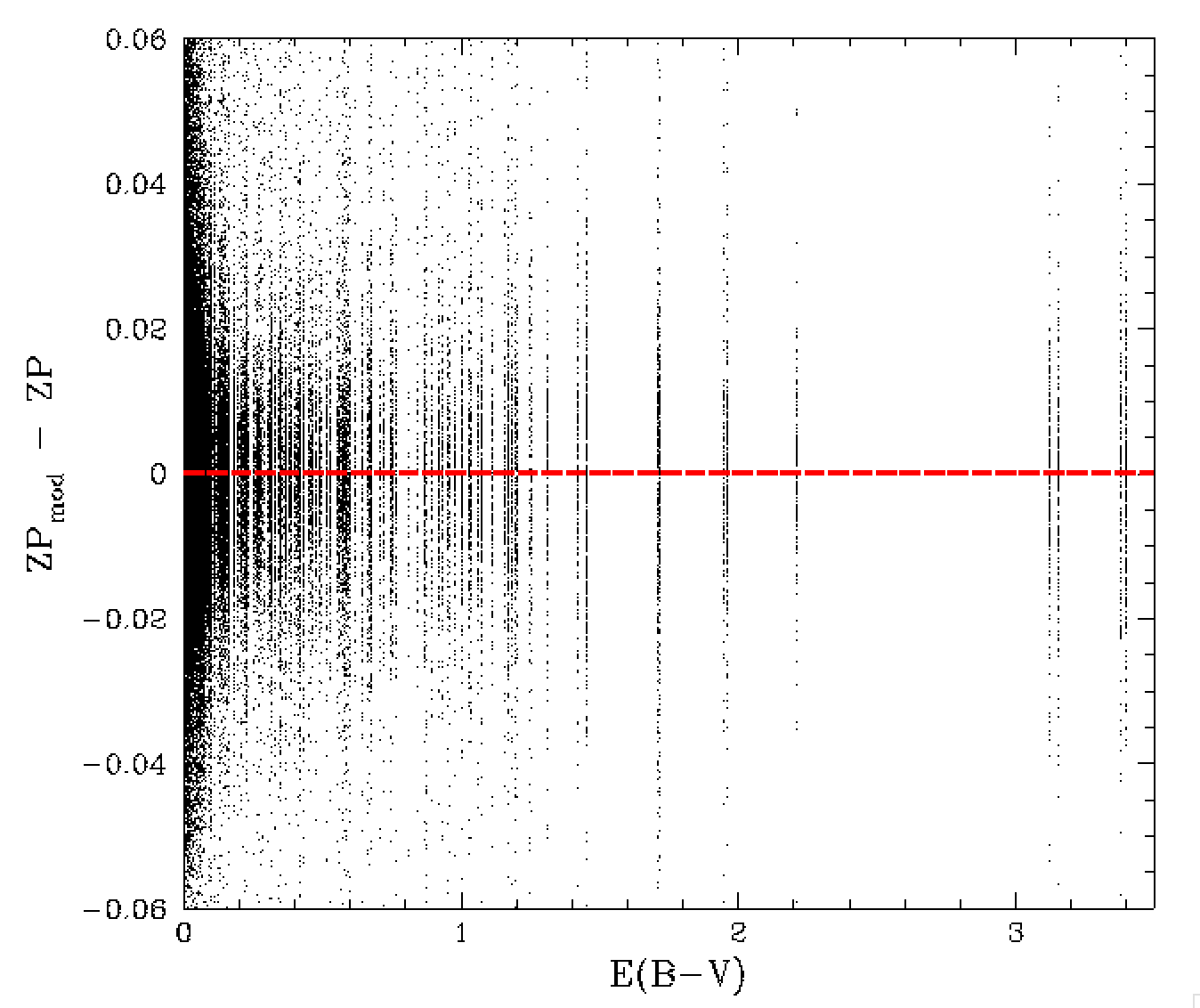
Residual differences between ZP and the ZP model for values of airmass and average quadrant reddening [E(B-V)].
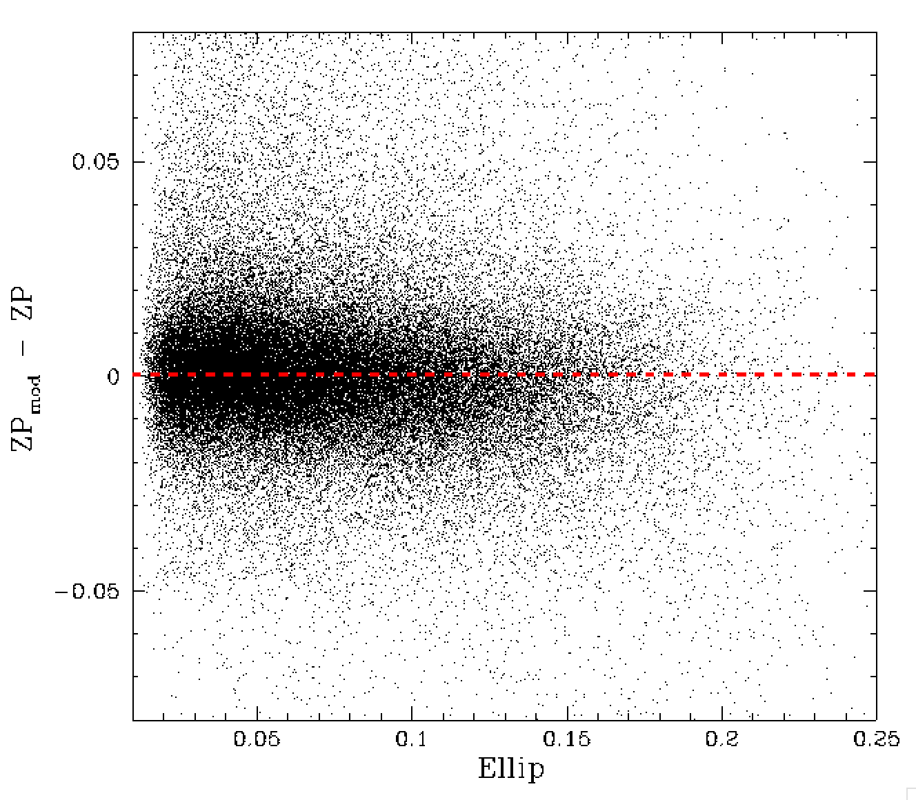
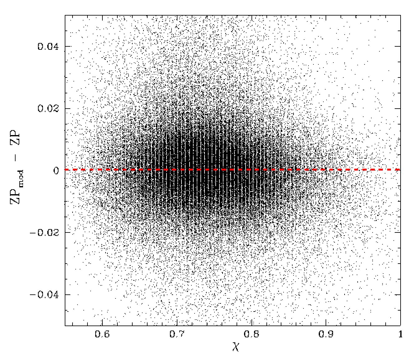
Residual differences between ZP and the ZP model for values of average frame ellipticity and PSF fit chi value.
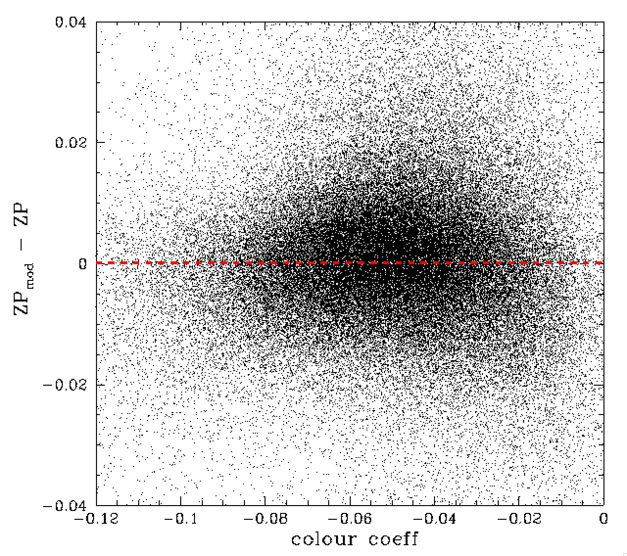
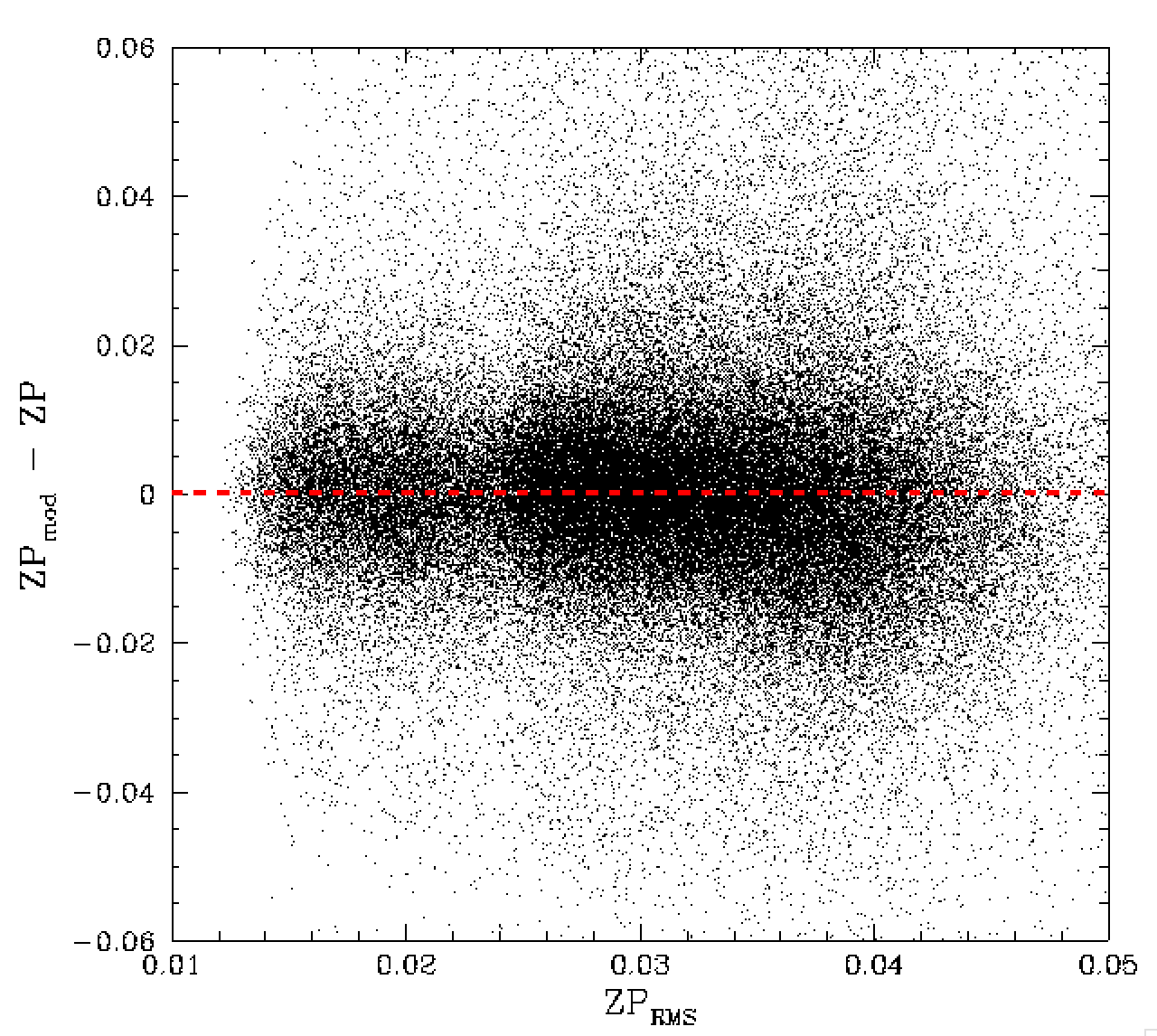
Residual differences between ZP and the ZP model for values of colour coefficient and ZPrms.
In the plots above appear to be most free of trends with the most important observables. As with the r-band data, we see that the ZPrms values from calibration fits appear to be overestimates. In this case there might be a slight trend.
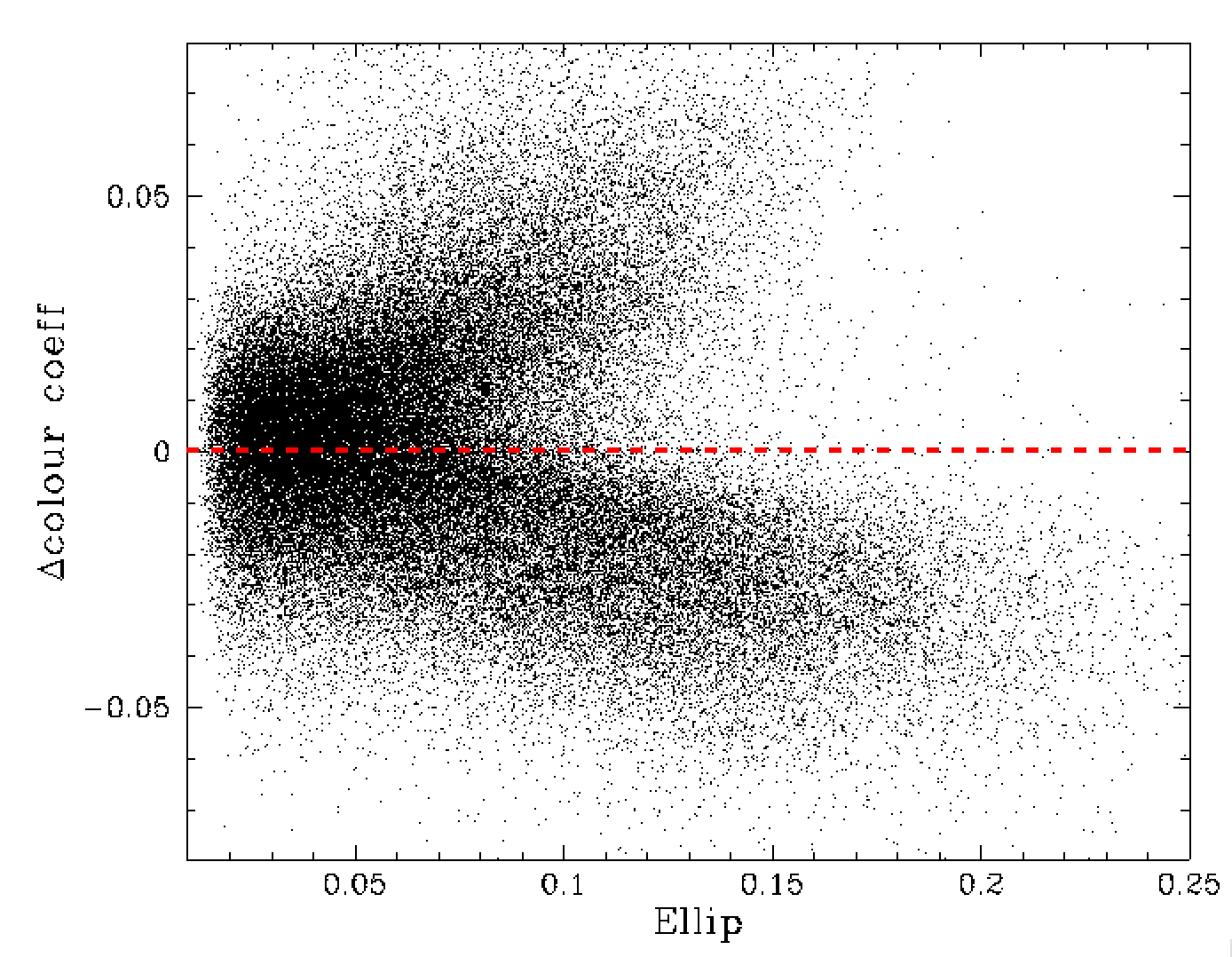
Variation in the colour coefficient relative to the median value for that field, vs the measured average ellipticity of the PSF sources in each image.
In the plot above we see that there is a very strong trend in ellipticity with the change in colour coefficients. This effect was also seen in r-band to lesser extent. This shows that variations in colour coefficents are strongly correlated to sources becoming increasingly elliptical. This is likely related to the strong dependence of PSF shape on colour. This was previously found to be particularly clear in the sharpness trend in g-band.
Conclusions
We have created a model for ZTF g-band ZP coefficients that is accurate to ~1%. The model is consistent with our r-band ZP model. In particular, the scale and phase of the time dependent structure is very similar. The main difference is the larger airmass in g-band dependence (as expected).Interestingly, the ZP data does not exhibit an obvious trend with skylevel as was previously seen in PS1 - ZTF g-band photometric residuals. However, the trend with source density is as evident as it is in r-band data. As with r-band data there is a strong colour trend with average ellipticity as well as slight but significant offsets between individual fields. Although we have only modelled one g-band channel it is likely that all other quadrants can be modelled to a similar level.